Q1:
Topic: Naïve Bayes Classifier

A patient goes to see a doctor. The doctor performs a test with 99% reliability - that is, 99% of people who are sick test positive and 99% of the healthy people test negative. The doctor knows that only 1 percent of the people in the country are sick. Now the question is: if the test comes out positive, is the probability of the patient actually being sick 99%?

Q2:
Topic: Naïve Bayes Classifier

We have two classes: “spam” and “ham” (not spam).

Training Data:

Class: Ham
D1: “good.”
D2: “very good.”

Class: Spam
D3: “bad.”
D4: “very bad.”
D5: “very bad, very bad.”

Test Data:
Identify the class for the following document:
D6: “good? bad! very bad!”

Q3:
Topic: Apriori Algorithm

TID : items_bought
T1 : { M,O,N,K,E,Y }
T2 : { D,O,N,K,E,Y }
T3 : { M,A,K,E }
T4 : { M,U,C,K,Y }
T5 : { C,O,O,K,I,E }

Let minimum support = 60%
And minimum confidence = 80%
Find all frequent item sets using Apriori.


Q4:
Topic: Decision Tree Induction

Create the decision tree for the following data:

Outlook,Temperature,Humidity,Wind,Play Tennis
Sunny,Hot,High,Weak,No
Sunny,Hot,High,Strong,No
Overcast,Hot,High,Weak,Yes
Rain,Mild,High,Weak,Yes
Rain,Cool,Normal,Weak,Yes
Rain,Cool,Normal,Strong,No
Overcast,Cool,Normal,Strong,Yes
Sunny,Mild,High,Weak,No
Sunny,Cool,Normal,Weak,Yes
Rain,Mild,Normal,Weak,Yes
Sunny,Mild,Normal,Strong,Yes
Overcast,Mild,High,Strong,Yes
Overcast,Hot,Normal,Weak,Yes
Rain,Mild,High,Strong,No

Q5:
For Iris Flower dataset, show the correlation plots for each pair of attributes.

Iris dataset comes in ARFF format alongside Weka tool.
Showing posts with label Weka. Show all posts
Showing posts with label Weka. Show all posts
Thursday, March 24, 2022
Machine Learning and Weka Interview (5 Questions)
Tuesday, March 15, 2022
Calculations for Info Gain and Gini Coefficient for Building Decision Tree
Formula For Calculating The Amount of Information in The Dataset
In plain English: Info(D) = (-1) times (summation of product of probability of class I and log of probability of class I) = Negative of summation of product of (probability of class I and log of probability of class I)Dataset
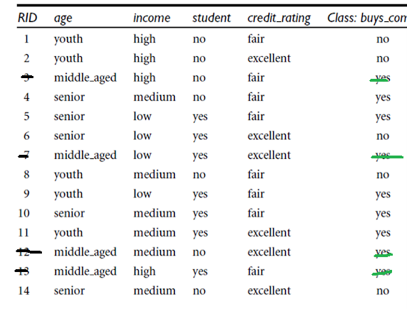
Class (buys_computer) Labels are: Yes and No How many Yes(s) are there: 9 No(s): 5 According to the formula and with log base 10: RHS = (-1) * ( ( (9/14) * log (9/14) ) + ( (5/14) * log (5/14) ) )With Log-Base-10: RHS = (-1) * ( ( (0.642) * log (0.642) ) + ( (0.357) * log (0.357) ) ) RHS = 0.283 With Log-Natural:With Log-Base-2:RHS = - ( 0.642 * ( -0.6374 ) ) - (( 0.357 ) * (-1.4854)) = 0.9394 Again, With Log-Base-10: RHS = (-1) * ( ( (0.642)* log (0.642) ) + ( (0.357) * log (0.357) ) ) = 0.283Information When We Split on Age
Age => Youth, Middle-aged, Senior Count of Youth => 5 Weight for youth => 5/14 Count of Middle-aged => 4 Weight for middle-aged => 4/14 Count of Senior => 5 Weight for Senior => 5/14 Component for YouthWith Log-Base-10: (5/14) * (-(3/5) * log (3/5) - (2/5) * log(2/5)) = 0.104 Component for middle-aged:(4/14) * ( -(4/4) * log (4/4) - 0/4 * log (0/4)) = 0 Component for senior:(5/14) * (-(3/5) * log (3/5) - (2/5) * log(2/5)) = 0.104 Information_when_we_split_on_age = 0.104 + 0 + 0.104 = 0.208 Information Gain When We Split on Age by Computation Using Log-Base-10: Info(D) - Info(on split by age) = 0.283 - 0.208 = 0.075WHAT HAPPENS WHEN WE SPLIT ON INCOME
Info(D) = 0.283 Weights for (High, Medium, and Low): High => 4/14 Medium => 6 / 14 Low => 4 / 14 Image for Income = High:Component for Income -> High = (4/14) * (-(2/4) * log (2/4) - (2/4) * log(2/4)) In Log base 10 Terms, it is: 0.086 Component for Income -> Medium =(6 /14) * (- (4/6) * log (4/6) - (2/6) * log (2/6)) = 0.118 Image for Income = Low:Component for Income -> Low = (4/14) * (-(3/4) * log(3/4) - (1/4) * log (1/4)) =0.0697 Info_when_split_on_income_for_log_base_10 = 0.086 + 0.118 + 0.0697 = 0.2737 Information Gain for Split on Age Log-Base-10 Was: Info(D) - Info(split of age) = 0.283 - 0.208 = 0.075 Information Gain for Split on Income Log-Base-10 Was: Info(D) - Info(split of Income) = 0.283 - 0.2737 = 0.0093 (Info(D) - Info(split of age)) > (Info(D) - Info(split of Income))CALCULATING INFORMATION GAIN WHEN WE SPLIT ON 'STUDENT'
'Student' Values are: Yes and No Weights for (Yes and No): Yes => 7/14 No => 7 / 14 Component for Student -> Yes =(7/14) * (-(6/7) * log(6/7) - (1/7) * log (1/7)) = 0.5 * (-0.8571 * log(0.8571) - 0.14285 * -0.8450) = 0.0890 Component for Student -> No =Component for Student -> No = (7/14) * ( -4/7 * (log 4/7) - 3/7 * log(3/7) ) = 0.054 Information (Student) = 0.0890 + 0.054 = 0.143 Information Gain = Info(D) - Info(Student) = 0.283 - 0.0890 = 0.194 Summarizing again: Information Gain for Age Log Base 10 Was: Info(D) - Info(split of age) = 0.283 - 0.208 = 0.075 Information Gain for Income Log Base 10 Was: Info(D) - Info(split of Income) = 0.283 - 0.2737 = 0.0093 Information Gain for Student with Log Base 10 was : Info(D) - Info(Student) = 0.283 - 0.194 = 0.089 We See: 0.089 > 0.075GINI INDEX COMPUTATION FOR ENTIRE DATASET
Class Label are: Yes and No How many Yes(s) are there: 9 How many No(s) are there: 5Gini(D) = 1 - (5/14)^2 - (9/14)^2 Gini(D) =0.4591 WHEN WE SPLIT ON AGE: Age => Youth, Middle-Aged, Senior Youth => 5 Weight for youth => 5/14 Middle-aged => 4 Weight for middle-aged => 4/14 Senior => 5 Weight for Senior => 5/14 For Youth:For Middle Aged:For Senior:Gini(when split on age) = (5/14) * (1 - (3/5) ^ 2 - (2/5) ^ 2 ) + (4/14) * (1 - (4/4)^2 - (0/4) ^ 2) + (5/14) * (1 - (2/5)^2 - (3/5)^2) = 0.342 Gini (when we split on income with classes {low, medium} and {high}) = = 0.714 * (1 - 0.49 - 0.09) + 0.285 * (1 - 0.0625 - 0.5625) = 0.406755 Gini(when split on 'Student' column) = 'Student' Values are: Yes and No Weights for (Yes and No): Yes => 7/14 No => 7 / 14 Component for Student -> Yes =(7/14) * (1 - (6/7)^2 - (1/7)^2) = 0.122 Component for Student -> No =(7/14) * (1 - (3/7)^2 - (4/7)^2) = 0.2448 Gini(when split on Student) = 0.122 + 0.2448 = 0.3668 Summarizing again for comparison Gini(when split on age) = 0.342 Gini (when we split on income with classes {low, medium} and {high}) = 0.406755 Gini(when split on Student) = 0.122 + 0.2448 = 0.3668 For 'Student' among (Age, Income and Student), Gini is the second lowest at 0.3668.Confusion Matrix
Decision Tree (J48) Report For 14 Txn Dataset From Weka
=== Run information === Scheme: weka.classifiers.trees.J48 -C 0.25 -M 2 Relation: 14_txn_buys_pc_numerical Instances: 14 Attributes: 5 age income student credet_rating class_buy_pc Test mode: 10-fold cross-validation === Classifier model (full training set) === J48 pruned tree ------------------ student <= 0 | age <= 0: no (3.0) | age > 0: yes (4.0/1.0) student > 0: yes (7.0/1.0) Number of Leaves : 3 Size of the tree : 5 Time taken to build model: 0.03 seconds === Stratified cross-validation === === Summary === Correctly Classified Instances 8 57.1429 % Incorrectly Classified Instances 6 42.8571 % Kappa statistic -0.0244 Mean absolute error 0.4613 Root mean squared error 0.5569 Relative absolute error 96.875 % Root relative squared error 112.8793 % Total Number of Instances 14 === Detailed Accuracy By Class === TP Rate FP Rate Precision Recall F-Measure MCC ROC Area PRC Area Class 0.200 0.222 0.333 0.200 0.250 -0.026 0.411 0.465 no 0.778 0.800 0.636 0.778 0.700 -0.026 0.411 0.662 yes Weighted Avg. 0.571 0.594 0.528 0.571 0.539 -0.026 0.411 0.592 === Confusion Matrix === a b <-- classified as 1 4 | a = no 2 7 | b = yesDecistion Tree Image For Buys a Computer or Not


Sunday, March 13, 2022
Interpretation of Decision Tree J48 output in Weka
Data Set Glimpse
@RELATION iris @ATTRIBUTE sepallength NUMERIC @ATTRIBUTE sepalwidth NUMERIC @ATTRIBUTE petallength NUMERIC @ATTRIBUTE petalwidth NUMERIC @ATTRIBUTE class {Iris-setosa,Iris-versicolor,Iris-virginica} The Data of the ARFF file looks like the following: @DATA 5.1,3.5,1.4,0.2,Iris-setosa 4.9,3.0,1.4,0.2,Iris-setosa 4.7,3.2,1.3,0.2,Iris-setosa 4.6,3.1,1.5,0.2,Iris-setosa 5.0,3.6,1.4,0.2,Iris-setosa ...=== Run information ===
Scheme: weka.classifiers.trees.J48 -C 0.25 -M 2 Relation: iris Instances: 150 Attributes: 5 sepallength sepalwidth petallength petalwidth class Test mode: 10-fold cross-validation === Classifier model (full training set) === J48 pruned tree ------------------ petalwidth <= 0.6: Iris-setosa (50.0) petalwidth > 0.6 | petalwidth <= 1.7 | | petallength <= 4.9: Iris-versicolor (48.0/1.0) | | petallength > 4.9 | | | petalwidth <= 1.5: Iris-virginica (3.0) | | | petalwidth > 1.5: Iris-versicolor (3.0/1.0) | petalwidth > 1.7: Iris-virginica (46.0/1.0) Number of Leaves : 5 Size of the tree : 9 Time taken to build model: 0.36 seconds === Stratified cross-validation === === Summary === Correctly Classified Instances 144 96 % Incorrectly Classified Instances 6 4 % Kappa statistic 0.94 Mean absolute error 0.035 Root mean squared error 0.1586 Relative absolute error 7.8705 % Root relative squared error 33.6353 % Total Number of Instances 150 === Detailed Accuracy By Class === TP Rate FP Rate Precision Recall F-Measure MCC ROC Area PRC Area Class 0.980 0.000 1.000 0.980 0.990 0.985 0.990 0.987 Iris-setosa 0.940 0.030 0.940 0.940 0.940 0.910 0.952 0.880 Iris-versicolor 0.960 0.030 0.941 0.960 0.950 0.925 0.961 0.905 Iris-virginica Weighted Avg. 0.960 0.020 0.960 0.960 0.960 0.940 0.968 0.924 === Confusion Matrix === a b c <-- classified as 49 1 0 | a = Iris-setosa 0 47 3 | b = Iris-versicolor 0 2 48 | c = Iris-virginicaInterpretation of Model Output From Weka
=== Confusion Matrix === a b c <-- classified as 49 1 0 | a = Iris-setosa 0 47 3 | b = Iris-versicolor 0 2 48 | c = Iris-virginica TRUE LABEL and CLASSIFIER LABEL: Data points classified as Setosa and are actually Setosa: 49 (True Positives) False Positives (predicted Setosa but are not Setosa): 0 False Negative: 1 True Negative: 47 + 3 + 2 + 48 = 100 When TRUE LABEL == CLASSIFIER LABEL => TRUE POSITIVES For Versicolor: True Positives: 47 False Positives: (1 + 2) = 3 False Negative: 3 True Negative: 49 + 48 For Virginica: True Positives: 48 False Positives: 3 False Negative: 2 (predicted as "not virginica" but were actually "virginica") True Negative: 49 + 1 + 47 Recall: How many of the setosa class were predicted as setosa? How many of data points belonging to class X were also predicted as X? Recall = (TP) / (TP + FN) For Setosa = 49 / 50 = 0.98 For Versicolor: 47 / 50 = 0.94 For Virginica: 48 / 50 = 0.96 Precision: How many of the total predictions of X were actually X? Precision = (TP) / (TP + FP) For Setosa = 49 / (49 + 0) = 1 For Versicolor = 47 / (47 + 3) = 0.940 For Virginica = 48 / (48 + 3) = 0.941

Wednesday, March 9, 2022
Interpretation of output from Weka for Apriori Algorithm
Our Dataset:

Best rules found in Weka using Apriori:
1. item5=t 2 ==> item1=t 2 <conf:(1)> lift:(1.5) lev:(0.07) [0] conv:(0.67) 2. item4=t 2 ==> item2=t 2 <conf:(1)> lift:(1.29) lev:(0.05) [0] conv:(0.44) 3. item5=t 2 ==> item2=t 2 <conf:(1)> lift:(1.29) lev:(0.05) [0] conv:(0.44) 4. item2=t item5=t 2 ==> item1=t 2 <conf:(1)> lift:(1.5) lev:(0.07) [0] conv:(0.67) 5. item1=t item5=t 2 ==> item2=t 2 <conf:(1)> lift:(1.29) lev:(0.05) [0] conv:(0.44) 6. item5=t 2 ==> item1=t item2=t 2 <conf:(1)> lift:(2.25) lev:(0.12) [1] conv:(1.11) 7. item1=t item4=t 1 ==> item2=t 1 <conf:(1)> lift:(1.29) lev:(0.02) [0] conv:(0.22) 8. item3=t item5=t 1 ==> item1=t 1 <conf:(1)> lift:(1.5) lev:(0.04) [0] conv:(0.33) 9. item3=t item5=t 1 ==> item2=t 1 <conf:(1)> lift:(1.29) lev:(0.02) [0] conv:(0.22) 10. item2=t item3=t item5=t 1 ==> item1=t 1 <conf:(1)> lift:(1.5) lev:(0.04) [0] conv:(0.33)Rule 1: item5=t 2 ==> item1=t 2 <conf:(1)> lift:(1.5) lev:(0.07) [0] conv:(0.67)
INTERPRETATION OF RULES:
item5=t 2
Meaning: item5 is in two transactions.item1=t 2
Meaning: item1 is in two transactions. Confidence(X -> Y) = P(Y | X) = (# txn with both X and Y) / (# txn with X) Lift = P(A and B) / (P(A) * P(B)) A -> item5 B -> item1 = (2/9) / ((2/9) * (6/9)) = 1.5 Conviction(X -> Y) = (1 - supp(Y)) / (1 - conf(X -> Y)) Support(X) => Support(item5) = 2/9 Support(Y) => Support(item1) = 6/9 Support(x -> Y) = 2 / 9 Confidence(item5 -> item1) = 1 Conviction(X -> Y) = (1 - (6/9)) / (1 - (1)) = Division by zero error Coverage (also called cover or LHS-support) is the support of the left-hand-side of the rule X => Y, i.e., supp(X). It represents a measure of to how often the rule can be applied. Coverage can be quickly calculated from the rule's quality measures (support and confidence) stored in the quality slot. Leverage computes the difference between the observed frequency of A and C appearing together and the frequency that would be expected if A and C were independent. A leverage value of 0 indicates independence. Leverage(A -> C) = support(A -> C) - support(A) * support(C) Range: [-1,1] Leverage(item5 -> item1) = support(item5 -> item1) - support(item5)*support(item5) Leverage(item5 -> item1) = (2/9) - (2/9)*(6/9) = 0.074Rule 2: item4=t 2 ==> item2=t 2 <conf:(1)> lift:(1.29) lev:(0.05) [0] conv:(0.44)
Confidence(X -> Y) = P(Y | X) (# of txns with Y and X) / (# of txns with X) X = item4 Y = item2 (# of txns with Y and X) = 2 (# of txns with item4) = 2 Confidence = 2/2 = 1 Lift = P(A and B) / (P(A) * P(B)) A = item4 B = item2 P(A and B) = (2/9) / ((2/9) * (7/9)) (P(A) * P(B)) = (2/9) * (7/9) Lift = (2/9) / ((2/9) * (7/9)) = 1.285Rule 10: item2=t item3=t item5=t 1 ==> item1=t 1 <conf:(1)> lift:(1.5) lev:(0.04) [0] conv:(0.33)
item2=t item3=t item5=t 1
Meaning: Items 2, 3 and 5 are appearing together in one transaction.item2=t item3=t item5=t 1 ==> item1=t 1
Meaning: Items 1, 2, 3 and 5 are appearing together in one transaction. Confidence(X -> Y) = P(Y | X) RHS = (# txn with both X and Y) / (# txn with X) = 1 / 1 = 1 Lift = P(A and B) / (P(A) * P(B)) = (1/9) / ((1/9) * (6/9)) = 1.5 Leverage(A -> C) = support(A -> C) - support(A) * support(C) support(Items 2, 3, 5) = 1/9 support(Item 1) = 6/9 support(Items 1, 2, 3, 5) = 1/9 Leverage(A -> C) = (1/9) - ((1/9) * (6/9)) = 0.037
Monday, March 7, 2022
Running Weka Apriori on 9_TXN_5_ITEMS Dataset
A CSV file not following Weka format of questions marks failed to load.
Error Message:

The File Erroneous For Weka is opening without any issues in LibreOffice:


tid,item1,item2,item3,item4,item5
T100,t,t,?,?,t
T200,?,t,?,t,?
T300,?,t,t,?,?
T400,t,t,?,t,?
T500,t,?,t,?,?
T600,?,t,t,?,?
T700,t,?,t,?,?
T800,t,t,t,?,t
T900,t,t,t,?,?
Weka's Apriori Run Information For Small Dataset As Above With TID
=== Run information ===

Scheme:       weka.associations.Apriori -N 10 -T 0 -C 0.9 -D 0.05 -U 1.0 -M 0.1 -S -1.0 -c -1
Relation:     9_txn_5_items
Instances:    9
Attributes:   6
                tid
                item1
                item2
                item3
                item4
                item5
=== Associator model (full training set) ===


Apriori
=======

Minimum support: 0.16 (1 instances)
Minimum metric <confidence>: 0.9
Number of cycles performed: 17

Generated sets of large itemsets:

Size of set of large itemsets L(1): 14

Size of set of large itemsets L(2): 31

Size of set of large itemsets L(3): 25

Size of set of large itemsets L(4): 8

Size of set of large itemsets L(5): 1

Best rules found:

1. item5=t 2 ==> item1=t 2    <conf:(1)> lift:(1.5) lev:(0.07) [0] conv:(0.67)
2. item4=t 2 ==> item2=t 2    <conf:(1)> lift:(1.29) lev:(0.05) [0] conv:(0.44)
3. item5=t 2 ==> item2=t 2    <conf:(1)> lift:(1.29) lev:(0.05) [0] conv:(0.44)
4. item2=t item5=t 2 ==> item1=t 2    <conf:(1)> lift:(1.5) lev:(0.07) [0] conv:(0.67)
5. item1=t item5=t 2 ==> item2=t 2    <conf:(1)> lift:(1.29) lev:(0.05) [0] conv:(0.44)
6. item5=t 2 ==> item1=t item2=t 2    <conf:(1)> lift:(2.25) lev:(0.12) [1] conv:(1.11)
7. tid=T100 1 ==> item1=t 1    <conf:(1)> lift:(1.5) lev:(0.04) [0] conv:(0.33)
8. tid=T100 1 ==> item2=t 1    <conf:(1)> lift:(1.29) lev:(0.02) [0] conv:(0.22)
9. tid=T100 1 ==> item5=t 1    <conf:(1)> lift:(4.5) lev:(0.09) [0] conv:(0.78)
10. tid=T200 1 ==> item2=t 1    <conf:(1)> lift:(1.29) lev:(0.02) [0] conv:(0.22)
We run the Apriori again without TID column this time:

Logs from Weka:
=== Run information ===

Scheme:       weka.associations.Apriori -N 10 -T 0 -C 0.9 -D 0.05 -U 1.0 -M 0.1 -S -1.0 -c -1
Relation:     9_txn_5_items_without_tid
Instances:    9
Attributes:   5
                item1
                item2
                item3
                item4
                item5
=== Associator model (full training set) ===


Apriori
=======

Minimum support: 0.16 (1 instances)
Minimum metric <confidence>: 0.9
Number of cycles performed: 17

Generated sets of large itemsets:

Size of set of large itemsets L(1): 5

Size of set of large itemsets L(2): 8

Size of set of large itemsets L(3): 5

Size of set of large itemsets L(4): 1

Best rules found:

1. item5=t 2 ==> item1=t 2    <conf:(1)> lift:(1.5) lev:(0.07) [0] conv:(0.67)
2. item4=t 2 ==> item2=t 2    <conf:(1)> lift:(1.29) lev:(0.05) [0] conv:(0.44)
3. item5=t 2 ==> item2=t 2    <conf:(1)> lift:(1.29) lev:(0.05) [0] conv:(0.44)
4. item2=t item5=t 2 ==> item1=t 2    <conf:(1)> lift:(1.5) lev:(0.07) [0] conv:(0.67)
5. item1=t item5=t 2 ==> item2=t 2    <conf:(1)> lift:(1.29) lev:(0.05) [0] conv:(0.44)
6. item5=t 2 ==> item1=t item2=t 2    <conf:(1)> lift:(2.25) lev:(0.12) [1] conv:(1.11)
7. item1=t item4=t 1 ==> item2=t 1    <conf:(1)> lift:(1.29) lev:(0.02) [0] conv:(0.22)
8. item3=t item5=t 1 ==> item1=t 1    <conf:(1)> lift:(1.5) lev:(0.04) [0] conv:(0.33)
9. item3=t item5=t 1 ==> item2=t 1    <conf:(1)> lift:(1.29) lev:(0.02) [0] conv:(0.22)
10. item2=t item3=t item5=t 1 ==> item1=t 1    <conf:(1)> lift:(1.5) lev:(0.04) [0] conv:(0.33)
Apriori Algorithm For Association Mining Using Weka's Supermarket Dataset
We will see that the 'Supermarket.arff' dataset from Weka Repository is a: Fixed columns, True-False Format


@relation supermarket
@attribute 'department1' { t}
@attribute 'department2' { t}
@attribute 'department3' { t}
@attribute 'department4' { t}
@attribute 'department5' { t}
@attribute 'department6' { t}
@attribute 'department7' { t}
@attribute 'department8' { t}
@attribute 'department9' { t}
@attribute 'grocery misc' { t}
@attribute 'department11' { t}
@attribute 'baby needs' { t}
@attribute 'bread and cake' { t}
@attribute 'baking needs' { t}
@attribute 'coupons' { t}
@attribute 'juice-sat-cord-ms' { t}
@attribute 'tea' { t}
@attribute 'biscuits' { t}
@attribute 'canned fish-meat' { t}
...
...
...
@attribute 'department215' { t}
@attribute 'department216' { t}
@attribute 'total' { low, high} % low < 100
@data
?,?,?,?,?,?,?,?,?,?,?,t,t,t,?,t,?,t,?,?,t,?,?,?,t,t,t,t,?,t,?,t,t,?,?,?,?,?,?,t,t,t,?,?,?,?,?,?,?,t,?,?,?,?,?,?,?,?,t,?,t,?,?,t,?,t,?,?,?,?,?,?,?,?,?,?,?,?,?,?,?,?,t,?,?,t,?,?,?,?,?,?,?,?,?,?,?,?,?,?,?,?,?,?,?,?,?,?,?,?,?,?,?,?,?,?,?,?,?,?,?,t,?,?,?,?,?,?,?,?,?,?,?,?,?,?,?,?,?,?,?,?,?,?,?,?,?,?,?,?,?,?,?,?,?,?,?,?,?,?,?,?,?,?,?,?,?,?,?,?,?,?,?,?,?,?,?,?,?,?,?,t,?,?,?,?,?,?,?,?,?,?,?,?,?,?,?,?,?,?,?,?,?,?,?,?,?,?,?,?,?,?,?,?,?,?,high
t,?,?,?,?,?,?,?,?,?,?,?,?,?,?,?,?,?,t,t,t,?,?,?,?,?,t,?,?,?,t,t,?,?,?,?,?,t,t,?,t,?,?,?,?,?,?,?,t,?,?,t,?,?,?,?,?,?,?,?,t,?,?,?,?,?,?,?,?,?,?,?,?,?,?,?,?,?,?,?,?,?,t,?,?,t,?,?,?,?,?,?,?,?,?,?,?,?,?,?,?,?,?,?,?,?,?,?,?,?,?,?,?,?,?,?,?,?,?,?,?,?,?,?,?,?,?,?,?,?,?,?,?,?,?,?,?,?,?,?,?,?,?,?,?,?,?,?,?,?,?,?,?,?,?,?,?,?,?,?,?,?,?,?,?,?,?,?,?,?,?,?,?,?,?,?,?,?,?,?,?,?,?,?,?,?,?,?,?,?,?,?,?,?,?,?,?,?,?,?,?,?,?,?,?,?,?,?,?,?,?,?,?,?,?,?,low
?,?,?,?,?,?,?,?,?,?,?,?,t,t,?,t,?,t,?,t,?,?,?,?,?,?,t,?,t,?,?,?,?,?,?,?,?,?,?,?,?,t,?,?,?,t,?,?,?,?,?,?,?,?,?,?,?,?,?,?,?,?,?,?,?,t,t,?,?,?,t,?,t,?,?,?,?,?,?,?,?,?,t,?,?,t,?,?,?,?,?,?,?,?,?,?,?,?,t,?,?,?,?,?,?,?,?,?,?,?,?,?,?,?,?,?,?,?,?,?,?,?,?,?,?,?,?,?,?,?,?,?,?,?,?,?,t,?,?,?,?,?,?,?,?,?,?,?,?,?,?,?,?,?,?,?,?,?,?,?,?,?,?,?,?,?,?,?,?,?,?,?,?,?,?,?,?,?,?,?,?,?,?,?,?,?,?,?,?,?,?,?,?,?,?,?,?,?,?,?,?,?,?,?,?,?,?,?,?,?,?,?,?,?,?,?,low
t,?,?,?,?,?,?,?,?,?,?,?,t,t,?,t,?,t,?,?,t,t,?,?,t,?,?,?,?,?,?,t,?,?,?,t,?,t,?,t,t,?,?,?,?,?,?,?,t,t,?,?,?,?,?,?,?,?,t,?,?,?,?,t,?,?,t,?,?,?,t,?,?,?,?,?,?,?,?,?,?,?,?,?,?,?,?,?,?,?,?,?,?,?,?,?,?,?,t,?,?,?,t,?,?,?,?,?,?,?,?,?,?,?,?,?,?,?,?,?,?,?,?,?,?,?,?,?,?,?,?,?,?,?,?,?,t,?,?,?,?,?,?,?,?,?,?,?,?,?,?,?,?,?,?,?,?,?,?,?,?,?,?,?,?,?,?,?,?,?,?,?,?,?,?,?,?,?,?,?,?,?,?,?,?,?,?,?,?,?,?,?,?,?,?,?,?,?,?,?,?,?,?,?,?,?,?,?,?,?,?,?,?,?,?,?,low
?,?,?,?,?,?,?,?,?,?,?,?,t,t,?,t,t,?,?,?,?,?,?,?,t,t,t,?,?,?,?,t,?,?,?,t,?,?,t,?,?,t,?,?,?,?,?,?,t,?,?,t,t,?,?,?,?,t,?,?,t,?,?,t,?,?,?,?,?,?,t,?,?,?,?,t,?,?,?,?,?,?,?,?,t,t,?,?,?,?,?,?,?,?,?,?,?,?,?,?,?,?,?,?,t,?,?,?,?,?,?,?,?,?,?,?,?,?,?,?,?,?,?,?,?,?,?,?,?,?,t,?,?,?,?,?,?,?,?,?,?,?,?,?,?,?,?,?,?,?,?,?,?,?,?,?,?,?,?,?,?,?,?,?,?,?,?,?,?,?,?,?,?,?,?,?,?,?,?,?,?,?,?,?,?,?,?,?,?,?,?,?,?,?,?,?,?,?,?,?,?,?,?,?,?,?,?,?,?,?,?,?,?,?,?,?,low
...
...
...
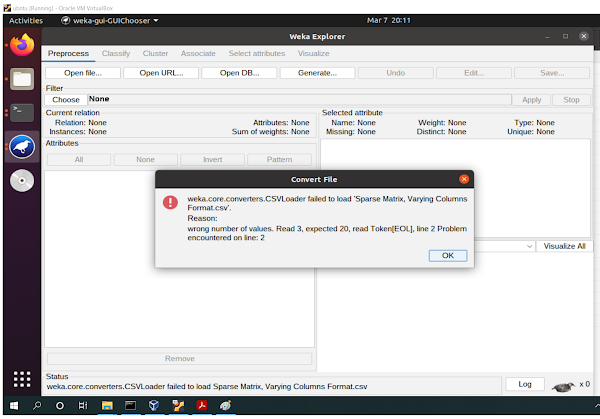
Error We Encountered in Weka When Loading "Sparse Matrix, Varying Columns Format" Input Format Dataset
IMG 1
IMG 2
Apriori Output in Weka For Supermarket Data
=== Run information ===

Scheme:       weka.associations.Apriori -N 10 -T 0 -C 0.9 -D 0.05 -U 1.0 -M 0.1 -S -1.0 -c -1
Relation:     supermarket
Instances:    4627
Attributes:   217
              [list of attributes omitted]
=== Associator model (full training set) ===


Apriori
=======

Minimum support: 0.15 (694 instances)
Minimum metric <confidence>: 0.9
Number of cycles performed: 17

Generated sets of large itemsets:

Size of set of large itemsets L(1): 44

Size of set of large itemsets L(2): 380

Size of set of large itemsets L(3): 910

Size of set of large itemsets L(4): 633

Size of set of large itemsets L(5): 105

Size of set of large itemsets L(6): 1

Best rules found:

 1. biscuits=t frozen foods=t fruit=t total=high 788 ==> bread and cake=t 723    <conf:(0.92)> lift:(1.27) lev:(0.03) [155] conv:(3.35)
 2. baking needs=t biscuits=t fruit=t total=high 760 ==> bread and cake=t 696    <conf:(0.92)> lift:(1.27) lev:(0.03) [149] conv:(3.28)
 3. baking needs=t frozen foods=t fruit=t total=high 770 ==> bread and cake=t 705    <conf:(0.92)> lift:(1.27) lev:(0.03) [150] conv:(3.27)
 4. biscuits=t fruit=t vegetables=t total=high 815 ==> bread and cake=t 746    <conf:(0.92)> lift:(1.27) lev:(0.03) [159] conv:(3.26)
 5. party snack foods=t fruit=t total=high 854 ==> bread and cake=t 779    <conf:(0.91)> lift:(1.27) lev:(0.04) [164] conv:(3.15)
 6. biscuits=t frozen foods=t vegetables=t total=high 797 ==> bread and cake=t 725    <conf:(0.91)> lift:(1.26) lev:(0.03) [151] conv:(3.06)
 7. baking needs=t biscuits=t vegetables=t total=high 772 ==> bread and cake=t 701    <conf:(0.91)> lift:(1.26) lev:(0.03) [145] conv:(3.01)
 8. biscuits=t fruit=t total=high 954 ==> bread and cake=t 866    <conf:(0.91)> lift:(1.26) lev:(0.04) [179] conv:(3)
 9. frozen foods=t fruit=t vegetables=t total=high 834 ==> bread and cake=t 757    <conf:(0.91)> lift:(1.26) lev:(0.03) [156] conv:(3)
10. frozen foods=t fruit=t total=high 969 ==> bread and cake=t 877    <conf:(0.91)> lift:(1.26) lev:(0.04) [179] conv:(2.92)
Subscribe to:
Posts (Atom)