From Mrs Indira to Dr Manmohan, we need to thank all PMs for rural development (Jun 2020)

Today, on 30th June 2020, the Prime Minister (Narendra Modi) briefly mentioned about the extent to which the government has supported the poor by providing them the ration in the difficult days of lockdown. It is remarkable that Indian government succeeded in feeding almost 80 crores people in India for more than 3 months for free. It is more than twice of the USA and European Union. Most of us might not look at this matter with surprise, but those who know that once India had “ship to mouth existence”, would certainly call it an achievement.
 
During the British Rule, more Indians were killed by the British policy of keeping the poor unfed than the direct massacre. Remember Churchill saying, “why hasn’t Gandhi died?”? The misery of India continued even after the independence because these things require time to improve. From Jawaharlal Nehru to Lal Bahadur Shastri, every Prime Minister stressed on the requirement of food security. In 1960’s, we had import food stocks to feed our population, which was increasing continuously. This type dependency on food over other countries raised questions on the sovereignty of India, every country which exported food stocks to India could dictate its terms and conditions. In that case, what was the point of attaining independence if we had to work as per the dictates of some other country?

First, remarkable, step was taken by the Prime Minister Indira Gandhi when she had launched ‘Green Revolution’. The revolution, to attain self sufficiency in terms of food security was an important matter for India’s sovereignty. The revolution was accepted by the masses and the agriculturalist with great enthusiasm. Every Prime Minister continued the principles underlined in the green revolution, which were – 

1. Income support to farmers through minimum support price
2. Creation of buffer stocks to deal with extraordinary situation
3. Normalisation of prices through sale of buffer stock time to time. 

Today, when the Prime Minister, releases the food stocks from the buffer stock of India, then we should be thankful to Mrs Gandhi for her initiation. Not only Mrs Gandhi but her trusted lieutenants in the battle like M. S. Swaminathan. 

It was during the reign of Atal Bihari Vajpayee that a mammoth task was undertaken by the government to create a network of metalled roads in every village. This required rural labourers. This spiralled up the labour demand in the rural area. Also, even the remotest village was now able to bring its produce to the markets which was not possible earlier because the transportation cost would have been much more than the production cost itself. 

During the reign of Dr Manmohan Singh, passing the legislation for the MGNREGA was another milestone, for which we should be thankful to him. Though, the programme went unsuccessful in the initial years from the economical perspective, but later on the government used it widely not only for the creation of the rural infrastructure but also the present government is eager to contain the migrant labourers within their village with the help of the scheme. 

Democracy is, in practice, a partisan exercise. When we bind ourselves with one particular political group, we tend to ignore the contribution of the others. This makes us myopic in our decision, and remember, we get the government we deserve. So next time, whenever you are told that nothing happened in the last 70 years, then you can answer that we achieved food security in last 70 years to the extent that the present Prime Minister can feed more the 80 crores population for more than 6 months. 

Step ahead? 
The present government has an equally important task to do when it comes to rural development. Today, many of the news articles and opinions talk about farmer suicide, but barely mention causes. Today, even after three decades of opening up our economy, we have kept our farmers under constraints. Every state government in the country, under the political pressure of middlemen, are afraid of taking any action for the welfare of the farmers, despite crying crocodilian tears for them in their election campaigns. 

To give freedom to the farmer, to sell his/her produce wherever she wants to, will be the least good we can do for her today. 

As per the current rules and regulation, any produce by the farmer needs to be sold in the nearest APMC Market. In that market, all the designated buyers must auction for the produce, but it is in theory. In practice, the designated buyers will make a cartel and would not buy the produce of a farmer more than the specified rate, which is extremely low. Sometimes, rates offered by the designated buyers is not sufficient to recover the basic cost. The farmer is bound to sell his produce there and nowhere else as per the state government laws. As a result, we see distress sales of farmers’ produce, resulting into farmer suicide. But the designated buyers, who get the produce at lowest minimum price from the farmer, sells the same commodity at maximum possible price in the market. Neither the final consumer is beneficiary nor is the farmer. Situation would have been different if the farmer was allowed to sell his produce directly to the consumer. 

Recent decision by the finance minister Nirmala Sitharaman is a welcome step in this direction. In her recent decisions, she made inter state commerce of agricultural goods beyond any restrictions of the draconian APMC act. Most of the state governments are not happy with the decision. Punjab government has expressed its refusal for this act as well. But for the larger good, this is a welcome step. 

Under Mrs. Indira Gandhi, we made initiations to attain food security. Under Mr. Vajpayee, we made strides in upgrading rural infrastructure. Under Dr Manmohan, we tried to check on the migration problem. Will we be able to look at the income security of the farmer under Modi regime? Only the time will tell. 

Credits: Shubham Rajput

Anomaly Detection Books (Jul 2020)

Download Books
    
1. Anomaly Detection Principles and Algorithms
Book by Chilukuri Krishna Mohan, HuaMing Huang, and Kishan G. Mehrotra

2. Practical Machine Learning: A New Look at Anomaly Detection
Book by Ellen Friedman and Ted Dunning

3. Beginning Anomaly Detection Using Python-Based Deep Learning: With Keras and PyTorch
Book by Sridhar Alla and Suman Kalyan Adari

4. Network Anomaly Detection: A Machine Learning Perspective
Book by Dhruba Kumar Bhattacharyya and Jugal Kalita

5. Anomaly Detection as a Service: Challenges, Advances, and Opportunities
Book
Originally published: 24 October 2017
Authors: Long Cheng, Xiaokui Shu, Salvatore J. Stolfo, Danfeng (Daphne) Yao

6. Applied Cloud Deep Semantic Recognition: Advanced Anomaly Detection
Book
Originally published: 2018

7. Outlier Analysis
Book by Charu C. Aggarwal
Originally published: 11 January 2013

8. Traffic Anomaly Detection
Book by Antonio Cua-Sánchez and J. Aracil

9. Outlier Ensembles: An Introduction
Book by Charu C. Aggarwal and Saket Sathe

10. Network Traffic Anomaly Detection and Prevention: Concepts, Techniques, and Tools
Book by Dhruba Kumar Bhattacharyya, Jugal Kalita, and Monowar H. Bhuyan

11. Machine Learning Methods for Behaviour Analysis and Anomaly Detection in Video
Book by Olga Isupova

12. Outlier Detection: Techniques and Applications: A Data Mining Perspective
Book by G. Athithan, M. Narasimha Murty, and N. N. R. Ranga Suri

13. Outlier Detection for Temporal Data
Book
Originally published: March 2014
Authors: Jing Gao, Manish Gupta, Charu C. Aggarwal, Jiawei Han

14. Machine Learning and Security: Protecting Systems with Data and Algorithms
Book by Clarence Chio and David Freeman

15. Data Mining: Concepts and Techniques
Book by Jiawei Han

16. Anomaly Detection Approach for Detecting Anomalies Using Netflow Records and ...
Book by Rajkumar Khatri

17. Smart Anomaly Detection for Sensor Systems: Computational Intelligence ...
Book by Antonio Liotta, Giovanni Iacca, and Hedde Bosman

18. Mobile Agent-Based Anomaly Detection and Verification System for Smart Home Sensor Networks
Book by Muhammad Usman, Surraya Khanum, and Xin-Wen Wu

19. Anomaly-Detection and Health-Analysis Techniques for Core Router Systems
Book
Originally published: 19 December 2019
Authors: Krishnendu Chakrabarty, Xinli Gu, Shi Jin, Zhaobo Zhang

20. Real-Time Progressive Hyperspectral Image Processing: Endmember Finding and Anomaly Detection
Book by Chein-I Chang

21. An Empirical Comparison of Monitoring Algorithms for Access Anomaly Detection
Book by Anne Dinning and Edith Schonberg

22. Anomaly Detection with an Application to Financial Data
Book by Fadi Barbara

23. Trace and Log Analysis: A Pattern Reference for Diagnostics and Anomaly ...
Book by Dmitry Vostokov

24. Robust Regression and Outlier Detection
Book by Annik Leroy and Peter Rousseeuw

25. The State of the Art in Intrusion Prevention and Detection
Book
Originally published: 2014

26. Applications of Data Mining in Computer Security
Book
Originally published: 31 May 2002

27. Finding Ghosts in Your Data: Anomaly Detection Techniques with Examples in Python
Kevin Feasel, 2022

Tags: Technology,Machine Learning,List of Books,

45 Years of Emergency (Jun 2020)

45 years of "from 12 AM tonight..." 
Since 2016, the words, "from 12 AM tonight..." are dreaded. The wrath of these words was also witnessed when the Prime Minister declared lockdown due to Covid-19 pandemic situation. But these words are not used by the current Prime Minister only, but many Prime Ministers in the past too, had fascination with these words. One such incident is of 26th June 1975, when, the then Prime Minister of India, on All India Radio declared that the President has declared emergency in the country at 12 AM tonight. 
Before jumping to the decision, rounds of meetings were held at the residence of Prime Minister Indira Gandhi and it was decided that the nation shall be put under the emergency at fortnight of 25th June 1975. [1]
But what this whole drama was about? Why such rounds of meetings were conducted at the PM residence with lawyers and Chief Minister of West Bengal, Siddharth Shankar Ray? [2]
To understand this, we need to go in the past, and understand how such a situation evolved in India and what was the outcome of it. Powerful leaders often fail to grasp the undercurrent of discontent prevailing in the masses, otherwise there had been no revolts in the past against powerful leaders. Something similar happened to Indira Gandhi. Mrs. Gandhi was fighting multiple fights at multiple fronts. She was fighting the discontent of masses due to rising unemployment, corruption in bureaucracy, poverty, interference in judiciary. At the same time the opposition, which consisted leaders like Atal Bihari Vajpayee, Chandra Shekhar, and the staunchest Morarji Desai, were making it difficult for her to survive the political battle. When all was not going well, a political veteran, hero of Quit India Movement, Loknayak Jayprakash Narayan had returned to the political scene and like never before a student agitation was launched against the Indira Government. The poems of Ramdhari Singh Dinkar, “singhasan khali karo, Janata aati hai”, meaning “vacate the power, the masses are coming”, were recited in the streets.
If that was not enough, Raj Narayan Singh, who had contested election against Indira Gandhi in Rae Bareilly, the famous Congress bastion, had filed a suit in the Allahabad High Court. It was alleged by Raj Narain Singh that Mrs. Gandhi had used government machinery in contesting her elections, which is not allowed even today. He alleged that not only Indira Gandhi used Indian Air Force planes to distribute pamplets but also Indian Army Jeep was used for election campaigning. The matter went to Allahabad High Court, and Justice Jaganmohan Sinha1 found Mrs. Gandhi guilty and asked her to vacate her seat. Also, Justice Sinha ordered Indira Gandhi to not to contest any election for coming six years. 

And the stage was set
To prevent the execution of the High Court decision, Article 356 of the Indian Constitution was invoked1. As per the Article, if there is any internal disturbance in the country, then the President can execute emergency in the country. The student agitation against Indira Gandhi was considered as the internal disturbance, and citing that, draft of an order was sent to the President of India, Fakhruddin Ali Ahmed, which he signed. Cartoonist Ranga came up with a satirical cartoon on this incidence. 



The cartoon depicting the President saying that “...if there are more ordinances, then tell them to wait” and he is shown busy in having bath. 

What emergency meant? 

The Constitution at that time was such that if Emergency is proclaimed, then all the Fundamental Rights of individuals shall be suspended [3]. It meant, that all the Fundamental Rights, including Article-21, which guaranteed “Right to Life” was suspended. Citizens no longer enjoyed any right to live, any time their life could be taken away from the government, and no citizen was able to go to the courts for the protection of their lives because Article-20 and Article-22 forbid [4] the Courts to consider any such petitions. 
In other words, an All Powerful Leader, who could do whatever she wish to, and there was no one to stop her. This is what happened. All leaders of opposition were sent to jailed except the leaders of Communist Party of India as they were not against Mrs. Gandhi at that time. Power supply to all the newspapers was stopped. Newspapers were allowed to print only what government allowed them to. Forceful and coercive means to control population were adopted. Even those who were unmarried, were arrested and vasectomy was conducted on them. [5] The sixteen point programme of Sanjay Gandhi was being implemented by state governments and there was no control on their powers to implement those. To conclude – democracy had died. 
When all of it was going on, instead of being apologetic to the atrocities, the Congress President D. K. Barua said in a public meeting that “India is Indira and Indira is India” [6]. It was reported in the report of Shah Commission, that police atrocities knew no limits. To add to the despair, if there was anyone who could protect people from the wrath of Mrs. Gandhi, then she was Mrs. Gandhi herself. While in jail, Lal Krishna Advani had written an opinion piece in which he compared to emergencies, which he mentioned in his autobiography, ‘My Country, My Life’ as well. It was something like...

In Germany in 1933, the Chancellor Hitler cited that there is a threat to the internal security, citing that there was an attempt to burn the Reichstag (German Parliament), therefore emergency was proclaimed. A majority was required to amend the constitution and to give all power to Hitler. To do so, all the opposition leaders were jailed. Then a law was passed that no judicial action can be taken on the actions of the Government. There shall be complete censorship of newspapers. A 25-point programme was launched for Germany (not 16-point, as it was in India) and a speech was given by S. Rudolf that, “Hitler is Germany, and Germany is Hitler, who takes oath to Hitler, takes Oath to Germany”. 

If you find it difficult to draw parallels between both the emergencies, then you must be intellectually very lazy. 

Why do we need to remember this today? 

There is a saying that, “those who don’t learn from history, are destined to doomed”. It is important to know how such things unfolded. Also, another important aspect of it, that those who claim legacy of Mrs. Gandhi, have not apologised even today for the actions she had taken. With what face we demand apology of British for the atrocities they did?  

References 
1. Turbulent Years – Pranab Mukherjee; India After Gandhi – Ramchandra Guha
2. Same sources as above. Source – My Country, My Life – L. K. Advani
3. Constitution of India – Durga Das Basu
4. Forbid In the sense that these rights prevent any arbitrary arrest and ensure proper judicial system. But these rights were suspended and therefore no judicial proceedings were required to arrest, detain, or even to kill someone. 
5. Shah Commission Report 
6. Turbulent Years – Pranab Mukherjee

Credits:
Shubham Rajput

What surrender looks like? (Jun 2020)

In the recent political jibe by the former President of the Indian National Congress Party, Mr. Rahul Gandhi, the Prime Minister of India, Mr. Narendra Modi was termed as ‘Surrender’ Modi, based on the assumption that Prime Minister has compromised the territorial integrity of the country. Many of the media reporters found it interesting that someone like Narendra Modi, for whom the territorial integrity is such an important aspect of his style of politics, can compromise on the territorial integrity. Therefore, for some media houses it was an opportunity to brand Narendra Modi as a weak Prime Minister and for some it was change in recipe they often served to their viewers. But for those who like to understand and consume facts more than the non sensical sensationalism provided by the news channels, it is important to know that what is surrender after all in the strategic times like these. 

To understand this, we need to understand what are the precedents in the history to compare the present circumstances.

Kashmir in 1948 

Just after the declaration of independence for Pakistan and partition of India, the Jammu and Kashmir princely state then ruled by Maharaja Hari Singh was in news. Pakistan wanted it to be the part of its territory and therefore sent Kabayalis to attack Jammu and Kashmir and incorporate it by force. Despite the repeated request of Sardar Vallabhbhai Patel, Indian army was not given permission to protect Kashmir from the plundering, murdering, loot, and rape crimes of Kabayalis. The point was that the Kashmir has not given its assent to join India. Was that the case? No! The Maharaja of the Jammu and Kashmir had given its assent to join India but Jawaharlal Nehru rejected that because he wanted Maharaja to remove his Prime Minister (then Jammu and Kashmir used to have a Prime Minister) Mehar Chand Mahajan and replace him with his friend Sheikh Abdullah. Do you call this as an example of surrender? Prime Minister of India let Kashmiri women raped, murdered, looted and plundered, just because his friend had not appointed his friend as the Prime Minister of the Jammu and Kashmir? If not surrender, then what is it?

All is not over yet. Even when somehow Sardar Patel managed to get the army enter in the Kashmir valley, more than half of the Jammu and Kashmir was captured by Pakistan. Just when Indian army was getting Kashmir free from Pakistan and pushing the Kabayali backwards, Pt. Nehru announced status quo. Which meant that whatever area Pakistan had annexed shall remain with Pakistan until United Nation sponsored solution is not accepted, which never came into being, and 1/3rd of Kashmir is still with the Pakistan. This is what we call surrender. 

Not a blade of grass grows there: 1962 

When China was pushing its army in the Indian Territory, then Prime Minister Jawaharlal Nehru told the Parliament to not worry much about Laddakh, not a single blade of grass grows there. And the descendants of that legacy are pointing out the surrender is an irony. In defence of Jawaharlal Nehru, maybe he knew about the war preparedness of the Indian army because his defence minister, V. K. Krishna Menon was busy in manufacturing utensils in the Ordinance factory. The defence capabilities were consistently lowered down by the defence minister Menon, who remained on that position for the longest time. This was the reason why Indian soldiers, who did not have any arms and ammunition to fight the Chinese incursion had to lose their lives. Much to the credit of the army, when Chinese government had released the official numbers of casualties on their side in 1962 war with India, in 1994, it was found that on some posts, more Chinese soldiers were killed by Indian, despite Indians had inferior or no arms with them. Major Shaitan Singh is said to have killed almost 100 soldiers with his bare hands. Nehru was getting regular signals that war is on the way, even then Nehru compromised on the national security. We lost 1/3rd territory of Laddakh. This is what surrender looks like. 

How to lose a war on table that is won on the battlefield: 1971-72 

The 1971 war for Pakistan is a war which no one wants to remember in Pakistan. Their country – East and West Pakistan were divided into two parts and a new country, Bangladesh, was forged out of it. Indian forces entered into the war on December 1st 1971, and concluded the war on December 16th 1971. The result of the 16-day war was partition of Pakistan and surrender of 90,000 Pakistani soldiers. The Prime Minister of the Pakistan, who was such a good actor, Bhutto, came to India with his daughter Benazir Bhutto to get their soldiers free. This was the golden opportunity with India to resolve the Kashmir issue for once and forever. Mrs. Indira Gandhi did almost contrary to that. Not only Mrs. Indira Gandhi gave 90,000 Pakistani soldiers to Pakistan in 1972, but also did not resolved the border dispute. She was in such a powerful position that she could have got all the Kashmir freed but what she did? She literally surrendered to the acting skills of Bhutto. That was a surrender. Moreover, we lost the 1971 war on the table. 

What is certainly not a surrender? 

The Chinese way or the Communist way to fight is to fight in the Salami tactics. They do not deliver the one and ultimate blow, instead they prefer to chop you piece by piece. Afterall that’s how they got control of China after the Civil War in China. To fight such battles, it is important to know that status quo is changed slowly and almost as important to intervene almost immediately, and not behave like V. K. Krishna Menon and Jawaharlal Nehru. India, in this context has been proactive. Not only the Indian soldiers were quick to intervene, but the kind of scar the Indian soldier left on their Chinese counterparts, it is unlikely that any such activity shall be pursued by the Chinese forces in the near future, except when there is no war. Also, the departure of the Army General to participate in the talks for the establishment of the status quo is a sign of swiftness of the Indian side. 

The Chinese did similar kind of activity in Doklam trijunction in 2016, when they were intercepted by the Indian side. China had to move backwards. It is evident from the way things are taking place that similar kind of outcome shall come after this whole standoff. And you don’t call this a surrender. You are forcing the Chinese to move backwards can certainly be not called as surrender. Question is, whether Mr. Rahul Gandhi will apologize if the Chinese army moved backwards and leave Finger-4? Or will he dare the Prime Minister to recover that area of Ladakh as well which was lost by his Great Grandfather in 1962? Or will he ask the Prime Minister to have control of those posts as well which his government from 2004-14 had given away to the Chinese side? 

Appendix 

Before the Kabayalis had attacked the J&K, Man Sing wanted to keep his princely status, he was on negotiation table with both India and Pakistan.

When the Kabayali attacked J&K, Hari Singh was ready to sign the instrument of accession. But Jawaharlal wanted that accession should be signed by the elected government under Sheikh Abdullah. Then replacement of Mehar Chand Mahajan with Sheikh Abdullah as Prime Minister, even if it was not democratic.

References 
% Wikipedia - Hari Singh

Credits:
Shubham Rajput

Working with skLearn's MinMax scaler and defining our own

We are going to try out scikit-learn's MinMaxScaler for two features of a dataset.

import pandas as pd
import numpy as np
from sklearn.preprocessing import MinMaxScaler

# Two lists with 20 values
train_df = pd.DataFrame({'A': list(range(1000, 3000, 100)), 'B': list(range(1000, 5000, 200))}) 

# Two lists with 42 values
test_df = pd.DataFrame({'A': list(range(-200, 4000, 100)), \
                        'B': sorted(list(range(1000, 4900, 100)) + [1050, 1150, 1250])}) 

scaler_a = MinMaxScaler(feature_range = (0, 10)) # feature_range: tuple (min, max), default=(0, 1)
scaler_b = MinMaxScaler(feature_range = (0, 10)) # feature_range: tuple (min, max), default=(0, 1)

train_df['a_skl'] = scaler_a.fit_transform(train_df[['A']])
train_df['b_skl'] = scaler_b.fit_transform(train_df[['B']])

print(train_df[0:1])
print(train_df[-1:])

Output:
       A     B  a_skl  b_skl
0  1000  1000    0.0    0.0
       A     B  a_skl  b_skl
19  2900  4800   10.0   10.0

test_df['a_skl'] = scaler_a.transform(test_df[['A']])
test_df['b_skl'] = scaler_b.transform(test_df[['B']])

print(test_df[0:1])
print(test_df[-1:])

Output:
    A     B     a_skl  b_skl
0 -200  1000 -6.315789    0.0
    A     B      a_skl  b_skl
41  3900  4800  15.263158   10.0

train_df_minmax_a = train_df['A'].agg([np.min, np.max])
train_df_minmax_b = train_df['B'].agg([np.min, np.max])

test_df_minmax_a = test_df['A'].agg([np.min, np.max])
test_df_minmax_b = test_df['B'].agg([np.min, np.max])

print(train_df_minmax_a)
print(train_df_minmax_b)

Output:

amin    1000
amax    2900
Name: A, dtype: int64

amin    1000
amax    4800
Name: B, dtype: int64

The problem

We have two features A and B. In training data, A has range: 1000 to 2900 and B has range: 1000 to 4800.
In test data, A has range: -200 to 3900, and B has range: 1000 to 4800.

On test data, B gets converted to values between 0 to 10 as specified in MinMaxScaler definition.
But A in test data gets converted to range: -6.3 to 15.26.

Result: A and B are still in different ranges on test data.

Fix

We should be able to anticipate the range we are going to observe in test data or in real time situation / production.
Next, we define a MinMaxScaler of our own.

For A, we set expected minimum to -500 and for B, we set expected minimum to 0. (Similarly for maximums.)

r_min = 0
r_max = 10

def getMinMax(cell, amin, amax):
    a = cell - amin
    x_std = a / (amax - amin)
    x_scaled = x_std * (r_max - r_min) + r_min
    return x_scaled 

test_df['a_gmm'] = test_df['A'].apply(lambda x: getMinMax(x, -500, train_df_minmax_a.amax))
test_df['b_gmm'] = test_df['B'].apply(lambda x: getMinMax(x, 800, train_df_minmax_b.amax))

print(test_df) 

Output:

      A       B       a_skl   b_skl   a_gmm   b_gmm
0	-200	1000	-6.31	0.00	0.88	0.50
1	-100	1050	-5.78	0.13	1.17	0.62
2	0   	1100	-5.26	0.26	1.47	0.75
...
39	3700	4600	14.21	9.47	12.35	9.50
40	3800	4700	14.73	9.73	12.64	9.75
41	3900	4800	15.26	10.0	12.94	10.0 

The way we have adjusted expected minimum value in test data, similarly we have to do for expected maximum to bring the scaled values in the same range. 

Issue fixed.

References

% https://scikit-learn.org/stable/modules/generated/sklearn.preprocessing.MinMaxScaler.html

% https://scikit-learn.org/stable/modules/generated/sklearn.preprocessing.minmax_scale.html

% https://scikit-learn.org/stable/auto_examples/preprocessing/plot_all_scaling.html

% https://scikit-learn.org/stable/modules/preprocessing.html

% https://benalexkeen.com/feature-scaling-with-scikit-learn/

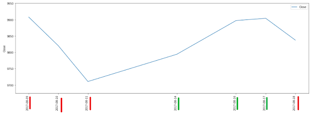
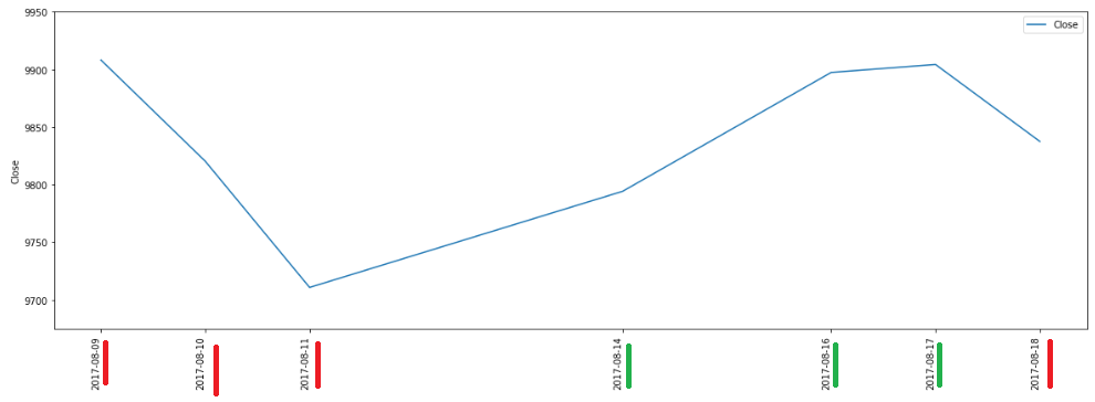
An exercise in visualization (plotting line plot and multicolored histogram with -ve and +ve values)

This post is an exercise in visualization (plotting line plot and multicolored histogram with -ve and +ve values). We will be using Pandas and Matplotlib libraries.

We are going to do plotting for a week of Nifty50 data from Aug 2017.

import pandas as pd

import matplotlib.pyplot as plt
import matplotlib.dates as mdates
%matplotlib inline

from dateutil import parser

df = pd.read_csv("files_1/201708.csv", encoding='utf8')
df['Change'] = 0
prev_close = 10114.65

def gen_change(row):
    global prev_close
    if row.Date == '01-Aug-2017':
        rtn_val = 0
    else:
        rtn_val = round(((row.Close - prev_close) / prev_close) * 100, 2)
        prev_close = row.Close
    return rtn_val

df.Change = df.apply(gen_change, axis = 1) 

We will plot for only a few dates of Aug 2017:

Line plot: 
subset_df = df[6:13]
plt.figure()
ax = subset_df[['Date', 'Close']].plot(figsize=(20,7))
ax.set_xticks(subset_df.index)
ax.set_ylim([9675, 9950])
ticklabels = plt.xticks(rotation=90)
plt.ylabel('Close')
plt.show() 




Multicolored Histogram for Negative and Positive values

negative_data = [x if x < 0 else 0 for x in list(subset_df.Change.values)]
positive_data = [x if x > 0 else 0 for x in list(subset_df.Change.values)]

fig = plt.figure()
ax = plt.subplot(111)
ax.bar(subset_df.Date.values, negative_data, width=1, color='r')
ax.bar(subset_df.Date.values, positive_data, width=1, color='g')
ticklabels = plt.xticks(rotation=90)
plt.xlabel('Date')
plt.ylabel('% Change')
plt.show()




Link to data file: Google Drive

Importance of posing right question for machine learning, data analysis and data preprocessing

We are going to demonstrate in this post the importance of posing the right question (presenting the ML use case, the ML problem correctly) and the importance of understanding data and presenting it to the ML model in the correct form.

The problem we are considering is of classification of data based on two columns, viz, alphabet and number.

+--------+------+------+
|alphabet|number|animal|
+--------+------+------+
|       A|     1|   Cat|
|       A|     3|   Cat|
|       A|     5|   Cat|
|       A|     7|   Cat|
|       A|     9|   Cat|
|       A|     0|   Dog|
|       A|     2|   Dog|
|       A|     4|   Dog|
|       A|     6|   Dog|
|       A|     8|   Dog|
|       B|     1|   Dog|
|       B|     3|   Dog|
|       B|     5|   Dog|
|       B|     7|   Dog|
|       B|     9|   Dog|
|       B|     0|   Cat|
|       B|     2|   Cat|
|       B|     4|   Cat|
|       B|     6|   Cat|
|       B|     8|   Cat|
+--------+------+------+

We have to tell if the "animal" is 'Cat' or 'Dog' based on 'alphabet' and 'number'. 
Rules are as follows:
If alphabet is A and number is odd, animal is cat.
If alphabet is A and number is even, animal is dog.
If alphabet is B and number is odd, animal is dog.
If alphabet is B and number is even, animal is cat.

We have written following "DecisionTreeClassifier" code for this task and we are going to see how the data preprocessing aids for this problem.

from pyspark import SparkContext
from pyspark.sql import SQLContext # Main entry point for DataFrame and SQL functionality.
from pyspark.ml import Pipeline

from pyspark.ml.classification import DecisionTreeClassifier
from pyspark.ml.feature import StringIndexer, VectorIndexer, OneHotEncoder
from pyspark.ml.evaluation import MulticlassClassificationEvaluator

sc = SparkContext.getOrCreate()
sqlCtx = SQLContext(sc)

a = list()
for i in range(0, 100000, 2):
 a.append(('A', i+1, 'Cat'))   
b = list()
for i in range(0, 100000, 2):
 a.append(('A', i, 'Dog'))   
c = list()
for i in range(0, 100000, 2):
 c.append(('B', i+1, 'Dog'))   
d = list()
for i in range(0, 100000, 2):
 d.append(('B', i, 'Cat'))   
 
l = a + b + c + d

df = sqlCtx.createDataFrame(l, ['alphabet', 'number', 'animal'])

alphabetIndexer = StringIndexer(inputCol="alphabet", outputCol="indexedAlphabet").fit(df)
df = alphabetIndexer.transform(df)

from pyspark.ml.feature import VectorAssembler

assembler = VectorAssembler(inputCols=["indexedAlphabet", "number"], outputCol="features")

# VectorAssembler does not have a "fit" method.
# VectorAssembler would not work on "alphabet" column directly. Throws the error: "IllegalArgumentException: Data type string of column alphabet is not supported". It would work on "indexedAlphabet".

df = assembler.transform(df)

# Index labels, adding metadata to the label column.
# Fit on whole dataset to include all labels in index.
labelIndexer = StringIndexer(inputCol="animal", outputCol="label").fit(df)

df = labelIndexer.transform(df)

dt = DecisionTreeClassifier(labelCol="label", featuresCol="features")

# Chain indexers and tree in a Pipeline
# pipeline = Pipeline(stages=[labelIndexer, featureIndexer, dt])
pipeline = Pipeline(stages=[dt])

# Split the data into training and test sets (30% held out for testing)
(trainingData, testData) = df.randomSplit([0.95, 0.05])

# Train model.  This also runs the indexers.
model = pipeline.fit(trainingData)

# Make predictions.
predictions = model.transform(testData)

# Select example rows to display.
# predictions.select("prediction", "label", "features").show()


# Select (prediction, true label) and compute test error
evaluator = MulticlassClassificationEvaluator(
    labelCol="label", predictionCol="prediction") # 'precision' and 'recall' for 'metricName' arg are invalid.

accuracy = evaluator.evaluate(predictions)
#print("Test Error = %g" % (1.0 - accuracy))
print(df.count())
print("Accuracy = %g" % (accuracy))

treeModel = model.stages[0]
print(treeModel) # summary only 

With this code, we observe the following results:

df.count(): 20000
Accuracy = 0.439774

df.count(): 200000
Accuracy = 0.471752

df.count(): 2000000
Accuracy = 0.490135 

What went wrong? 

We posed a simple classification problem to DecisionTreeClassifier, but we did not simplify the data to turn numbers into 'odd or even' indicator. This makes the learning so hard for model that with even 2 million data points, the classification accuracy stood at 49%.

~ ~ ~

Code changes to produce simplified data:
Change 1: replacing 'number' with 'odd or even' indicator.
Change 2: reducing number of data points.

a = list()
for i in range(0, 1000, 2):
 a.append(('A', (i+1) % 2, 'Cat'))   
b = list()
for i in range(0, 1000, 2):
 a.append(('A', i%2, 'Dog'))   
c = list()
for i in range(0, 1000, 2):
 c.append(('B', (i+1) % 2, 'Dog'))   
d = list()
for i in range(0, 1000, 2):
 d.append(('B', i%2, 'Cat'))
 
Result:

df.count(): 200
Accuracy = 0.228571

df.count(): 2000
Accuracy = 1 

Technology Listing related to Deep Learning (Jun 2020)

1. BIOS 

BIOS (pronounced: /ˈbaɪɒs/, BY-oss; an acronym for Basic Input/Output System and also known as the System BIOS, ROM BIOS or PC BIOS) is firmware used to perform hardware initialization during the booting process (power-on startup), and to provide runtime services for operating systems and programs. The BIOS firmware comes pre-installed on a personal computer's system board, and it is the first software to run when powered on. The name originates from the Basic Input/Output System used in the CP/M operating system in 1975. The BIOS originally proprietary to the IBM PC has been reverse engineered by companies looking to create compatible systems. The interface of that original system serves as a de facto standard.

The BIOS in modern PCs initializes and tests the system hardware components, and loads a boot loader from a mass memory device which then initializes an operating system. In the era of DOS, the BIOS provided a hardware abstraction layer for the keyboard, display, and other input/output (I/O) devices that standardized an interface to application programs and the operating system. More recent operating systems do not use the BIOS after loading, instead accessing the hardware components directly.

Most BIOS implementations are specifically designed to work with a particular computer or motherboard model, by interfacing with various devices that make up the complementary system chipset. Originally, BIOS firmware was stored in a ROM chip on the PC motherboard. In modern computer systems, the BIOS contents are stored on flash memory so it can be rewritten without removing the chip from the motherboard. This allows easy, end-user updates to the BIOS firmware so new features can be added or bugs can be fixed, but it also creates a possibility for the computer to become infected with BIOS rootkits. Furthermore, a BIOS upgrade that fails can brick the motherboard permanently, unless the system includes some form of backup for this case.

Unified Extensible Firmware Interface (UEFI) is a successor to the legacy PC BIOS, aiming to address its technical shortcomings.



Ref: BIOS

2. Unified Extensible Firmware Interface (UEFI) 

The Unified Extensible Firmware Interface (UEFI) is a specification that defines a software interface between an operating system and platform firmware. UEFI replaces the legacy Basic Input/Output System (BIOS) firmware interface originally present in all IBM PC-compatible personal computers, with most UEFI firmware implementations providing support for legacy BIOS services. UEFI can support remote diagnostics and repair of computers, even with no operating system installed.

Intel developed the original Extensible Firmware Interface (EFI) specifications. Some of the EFI's practices and data formats mirror those of Microsoft Windows. In 2005, UEFI deprecated EFI 1.10 (the final release of EFI). The Unified EFI Forum is the industry body that manages the UEFI specifications throughout.

EFI's position in the software stack:


History
The original motivation for EFI came during early development of the first Intel–HP Itanium systems in the mid-1990s. BIOS limitations (such as 16-bit processor mode, 1 MB addressable space and PC AT hardware) had become too restrictive for the larger server platforms Itanium was targeting. The effort to address these concerns began in 1998 and was initially called Intel Boot Initiative. It was later renamed to Extensible Firmware Interface (EFI).

In July 2005, Intel ceased its development of the EFI specification at version 1.10, and contributed it to the Unified EFI Forum, which has developed the specification as the Unified Extensible Firmware Interface (UEFI). The original EFI specification remains owned by Intel, which exclusively provides licenses for EFI-based products, but the UEFI specification is owned by the UEFI Forum.

Version 2.0 of the UEFI specification was released on 31 January 2006. It added cryptography and "secure boot". Version 2.1 of the UEFI specification was released on 7 January 2007. It added network authentication and the user interface architecture ('Human Interface Infrastructure' in UEFI). The latest UEFI specification, version 2.8, was approved in March 2019.

Tiano was the first open source UEFI implementation and was released by Intel in 2004. Tiano has since then been superseded by EDK and EDK2 and is now maintained by the TianoCore community.

In December 2018, Microsoft announced Project Mu, a fork of TianoCore EDK2 used in Microsoft Surface and Hyper-V products. The project promotes the idea of Firmware as a Service.

Advantages
The interface defined by the EFI specification includes data tables that contain platform information, and boot and runtime services that are available to the OS loader and OS. UEFI firmware provides several technical advantages over a traditional BIOS system:

1. Ability to use large disks partitions (over 2 TB) with a GUID Partition Table (GPT)
2. CPU-independent architecture
3. CPU-independent drivers
4. Flexible pre-OS environment, including network capability
5. Modular design
6. Backward and forward compatibility

Ref: UEFI

3. Serial ATA 

Serial ATA (SATA, abbreviated from Serial AT Attachment) is a computer bus interface that connects host bus adapters to mass storage devices such as hard disk drives, optical drives, and solid-state drives. Serial ATA succeeded the earlier Parallel ATA (PATA) standard to become the predominant interface for storage devices.

Serial ATA industry compatibility specifications originate from the Serial ATA International Organization (SATA-IO) which are then promulgated by the INCITS Technical Committee T13, AT Attachment (INCITS T13).

History
SATA was announced in 2000 in order to provide several advantages over the earlier PATA interface such as reduced cable size and cost (seven conductors instead of 40 or 80), native hot swapping, faster data transfer through higher signaling rates, and more efficient transfer through an (optional) I/O queuing protocol.

Serial ATA industry compatibility specifications originate from the Serial ATA International Organization (SATA-IO). The SATA-IO group collaboratively creates, reviews, ratifies, and publishes the interoperability specifications, the test cases and plugfests. As with many other industry compatibility standards, the SATA content ownership is transferred to other industry bodies: primarily INCITS T13 and an INCITS T10 subcommittee (SCSI), a subgroup of T10 responsible for Serial Attached SCSI (SAS). The remainder of this article strives to use the SATA-IO terminology and specifications.

Before SATA's introduction in 2000, PATA was simply known as ATA. The "AT Attachment" (ATA) name originated after the 1984 release of the IBM Personal Computer AT, more commonly known as the IBM AT. The IBM AT's controller interface became a de facto industry interface for the inclusion of hard disks. "AT" was IBM's abbreviation for "Advanced Technology"; thus, many companies and organizations indicate SATA is an abbreviation of "Serial Advanced Technology Attachment". However, the ATA specifications simply use the name "AT Attachment", to avoid possible trademark issues with IBM.

SATA host adapters and devices communicate via a high-speed serial cable over two pairs of conductors. In contrast, parallel ATA (the redesignation for the legacy ATA specifications) uses a 16-bit wide data bus with many additional support and control signals, all operating at a much lower frequency. To ensure backward compatibility with legacy ATA software and applications, SATA uses the same basic ATA and ATAPI command sets as legacy ATA devices.

SATA has replaced parallel ATA in consumer desktop and laptop computers; SATA's market share in the desktop PC market was 99% in 2008. PATA has mostly been replaced by SATA for any use; with PATA in declining use in industrial and embedded applications that use CompactFlash (CF) storage, which was designed around the legacy PATA standard. A 2008 standard, CFast to replace CompactFlash is based on SATA.

Features
1. Hot plug
2. Advanced Host Controller Interface

Ref: Serial ATA

4. Hard disk drive interface 

Hard disk drives are accessed over one of a number of bus types, including parallel ATA (PATA, also called IDE or EIDE; described before the introduction of SATA as ATA), Serial ATA (SATA), SCSI, Serial Attached SCSI (SAS), and Fibre Channel. Bridge circuitry is sometimes used to connect hard disk drives to buses with which they cannot communicate natively, such as IEEE 1394, USB, SCSI and Thunderbolt.

Ref: HDD Interface

5. Solid-state drive 

A solid-state drive (SSD) is a solid-state storage device that uses integrated circuit assemblies to store data persistently, typically using flash memory, and functioning as secondary storage in the hierarchy of computer storage. It is also sometimes called a solid-state device or a solid-state disk, even though SSDs lack the physical spinning disks and movable read–write heads used in hard drives ("HDD") or floppy disks.

% While the price of SSDs has continued to decline over time, SSDs are (as of 2020) still more expensive per unit of storage than HDDs and are expected to remain so into the next decade.

% SSDs based on NAND Flash will slowly leak charge over time if left for long periods without power. This causes worn-out drives (that have exceeded their endurance rating) to start losing data typically after one year (if stored at 30 °C) to two years (at 25 °C) in storage; for new drives it takes longer. Therefore, SSDs are not suitable for archival storage. 3D XPoint is a possible exception to this rule, however it is a relatively new technology with unknown long-term data-retention characteristics.

Improvement of SSD characteristics over time
Parameter  Started with (1991)   Developed to (2018)                Improvement
Capacity   20 megabytes	         100 terabytes (Nimbus Data DC100)	5-million-to-one
Price	   US$50 per megabyte	 US$0.372 per gigabyte (Samsung PM1643)	134,408-to-one

Ref: Solid-state drive

6. CUDA 

CUDA (Compute Unified Device Architecture) is a parallel computing platform and application programming interface (API) model created by Nvidia. It allows software developers and software engineers to use a CUDA-enabled graphics processing unit (GPU) for general purpose processing – an approach termed GPGPU (General-Purpose computing on Graphics Processing Units). The CUDA platform is a software layer that gives direct access to the GPU's virtual instruction set and parallel computational elements, for the execution of compute kernels.

The CUDA platform is designed to work with programming languages such as C, C++, and Fortran. This accessibility makes it easier for specialists in parallel programming to use GPU resources, in contrast to prior APIs like Direct3D and OpenGL, which required advanced skills in graphics programming. CUDA-powered GPUs also support programming frameworks such as OpenACC and OpenCL; and HIP by compiling such code to CUDA. When CUDA was first introduced by Nvidia, the name was an acronym for Compute Unified Device Architecture, but Nvidia subsequently dropped the common use of the acronym.

Ref: CUDA

7. Graphics Processing Unit 

A graphics processing unit (GPU) is a specialized electronic circuit designed to rapidly manipulate and alter memory to accelerate the creation of images in a frame buffer intended for output to a display device. GPUs are used in embedded systems, mobile phones, personal computers, workstations, and game consoles. Modern GPUs are very efficient at manipulating computer graphics and image processing. Their highly parallel structure makes them more efficient than general-purpose central processing units (CPUs) for algorithms that process large blocks of data in parallel. In a personal computer, a GPU can be present on a video card or embedded on the motherboard. In certain CPUs, they are embedded on the CPU die.

The term "GPU" was coined by Sony in reference to the PlayStation console's Toshiba-designed Sony GPU in 1994. The term was popularized by Nvidia in 1999, who marketed the GeForce 256 as "the world's first GPU". It was presented as a "single-chip processor with integrated transform, lighting, triangle setup/clipping, and rendering engines". Rival ATI Technologies coined the term "visual processing unit" or VPU with the release of the Radeon 9700 in 2002.

GPU companies 
Many companies have produced GPUs under a number of brand names. In 2009, Intel, Nvidia and AMD/ATI were the market share leaders, with 49.4%, 27.8% and 20.6% market share respectively. However, those numbers include Intel's integrated graphics solutions as GPUs. Not counting those, Nvidia and AMD control nearly 100% of the market as of 2018. Their respective market shares are 66% and 33%. In addition, S3 Graphics and Matrox produce GPUs. Modern smartphones also use mostly Adreno GPUs from Qualcomm, PowerVR GPUs from Imagination Technologies and Mali GPUs from ARM.

~ ~ ~

% Modern GPUs use most of their transistors to do calculations related to 3D computer graphics. In addition to the 3D hardware, today's GPUs include basic 2D acceleration and framebuffer capabilities (usually with a VGA compatibility mode). Newer cards such as AMD/ATI HD5000-HD7000 even lack 2D acceleration; it has to be emulated by 3D hardware. GPUs were initially used to accelerate the memory-intensive work of texture mapping and rendering polygons, later adding units to accelerate geometric calculations such as the rotation and translation of vertices into different coordinate systems. Recent developments in GPUs include support for programmable shaders which can manipulate vertices and textures with many of the same operations supported by CPUs, oversampling and interpolation techniques to reduce aliasing, and very high-precision color spaces. Because most of these computations involve matrix and vector operations, engineers and scientists have increasingly studied the use of GPUs for non-graphical calculations; they are especially suited to other embarrassingly parallel problems.

% With the emergence of deep learning, the importance of GPUs has increased. In research done by Indigo, it was found that while training deep learning neural networks, GPUs can be 250 times faster than CPUs. The explosive growth of Deep Learning in recent years has been attributed to the emergence of general purpose GPUs. There has been some level of competition in this area with ASICs, most prominently the Tensor Processing Unit (TPU) made by Google. However, ASICs require changes to existing code and GPUs are still very popular.

Ref: GPU

8. Tensor processing unit

A tensor processing unit (TPU) is an AI accelerator application-specific integrated circuit (ASIC) developed by Google specifically for neural network machine learning, particularly using Google's own TensorFlow software. Google began using TPUs internally in 2015, and in 2018 made them available for third party use, both as part of its cloud infrastructure and by offering a smaller version of the chip for sale.

Edge TPU

This article's use of external links may not follow Wikipedia's policies or guidelines. Please improve this article by removing excessive or inappropriate external links, and converting useful links where appropriate into footnote references. (March 2020) (Learn how and when to remove this template message)
In July 2018, Google announced the Edge TPU. The Edge TPU is Google's purpose-built ASIC chip designed to run machine learning (ML) models for edge computing, meaning it is much smaller and consumes far less power compared to the TPUs hosted in Google datacenters (also known as Cloud TPUs). In January 2019, Google made the Edge TPU available to developers with a line of products under the Coral brand. The Edge TPU is capable of 4 trillion operations per second while using 2W.

The product offerings include a single board computer (SBC), a system on module (SoM), a USB accessory, a mini PCI-e card, and an M.2 card. The SBC Coral Dev Board and Coral SoM both run Mendel Linux OS – a derivative of Debian. The USB, PCI-e, and M.2 products function as add-ons to existing computer systems, and support Debian-based Linux systems on x86-64 and ARM64 hosts (including Raspberry Pi).

The machine learning runtime used to execute models on the Edge TPU is based on TensorFlow Lite. The Edge TPU is only capable of accelerating forward-pass operations, which means it's primarily useful for performing inferences (although it is possible to perform lightweight transfer learning on the Edge TPU). The Edge TPU also only supports 8-bit math, meaning that for a network to be compatible with the Edge TPU, it needs to be trained using TensorFlow quantization-aware training technique.

On November 12, 2019, Asus announced a pair of single-board computer (SBCs) featuring the Edge TPU. The Asus Tinker Edge T and Tinker Edge R Board designed for IoT and edge AI. The SBCs support Android and Debian operating systems. ASUS has also demoed a mini PC called Asus PN60T featuring the Edge TPU.

On January 2, 2020, Google announced the Coral Accelerator Module and Coral Dev Board Mini, to be demoed at CES 2020 later the same month. The Coral Accelerator Module is a multi-chip module featuring the Edge TPU, PCIe and USB interfaces for easier integration. The Coral Dev Board Mini is a smaller SBC featuring the Coral Accelerator Module and MediaTek 8167s SoC.

Ref: TPU

9. PyTorch

PyTorch is an open source machine learning library based on the Torch library, used for applications such as computer vision and natural language processing, primarily developed by Facebook's AI Research lab (FAIR). It is free and open-source software released under the Modified BSD license. Although the Python interface is more polished and the primary focus of development, PyTorch also has a C++ interface.

A number of pieces of Deep Learning software are built on top of PyTorch, including Tesla, Uber's Pyro, HuggingFace's Transformers, and Catalyst.

PyTorch provides two high-level features:

# Tensor computing (like NumPy) with strong acceleration via graphics processing units (GPU)
# Deep neural networks built on a tape-based automatic differentiation system

PyTorch tensors:
PyTorch defines a class called Tensor (torch.Tensor) to store and operate on homogeneous multidimensional rectangular arrays of numbers. PyTorch Tensors are similar to NumPy Arrays, but can also be operated on a CUDA-capable Nvidia GPU. PyTorch supports various sub-types of Tensors.

History:

Facebook operates both PyTorch and Convolutional Architecture for Fast Feature Embedding (Caffe2), but models defined by the two frameworks were mutually incompatible. The Open Neural Network Exchange (ONNX) project was created by Facebook and Microsoft in September 2017 for converting models between frameworks. Caffe2 was merged into PyTorch at the end of March 2018.

Ref: PyTorch

10. TensorFlow

TensorFlow is a free and open-source software library for dataflow and differentiable programming across a range of tasks. It is a symbolic math library, and is also used for machine learning applications such as neural networks. It is used for both research and production at Google.‍

TensorFlow was developed by the Google Brain team for internal Google use. It was released under the Apache License 2.0 on November 9, 2015.

~ ~ ~

TensorFlow is Google Brain's second-generation system. Version 1.0.0 was released on February 11, 2017. While the reference implementation runs on single devices, TensorFlow can run on multiple CPUs and GPUs (with optional CUDA and SYCL extensions for general-purpose computing on graphics processing units). TensorFlow is available on 64-bit Linux, macOS, Windows, and mobile computing platforms including Android and iOS.

Its flexible architecture allows for the easy deployment of computation across a variety of platforms (CPUs, GPUs, TPUs), and from desktops to clusters of servers to mobile and edge devices.

TensorFlow computations are expressed as stateful dataflow graphs. The name TensorFlow derives from the operations that such neural networks perform on multidimensional data arrays, which are referred to as tensors. During the Google I/O Conference in June 2016, Jeff Dean stated that 1,500 repositories on GitHub mentioned TensorFlow, of which only 5 were from Google.

In December 2017, developers from Google, Cisco, RedHat, CoreOS, and CaiCloud introduced Kubeflow at a conference. Kubeflow allows operation and deployment of TensorFlow on Kubernetes.

In March 2018, Google announced TensorFlow.js version 1.0 for machine learning in JavaScript.

In Jan 2019, Google announced TensorFlow 2.0. It became officially available in Sep 2019.

In May 2019, Google announced TensorFlow Graphics for deep learning in computer graphics.

Ref: TensorFlow

11. Theano (software)

Theano is a Python library and optimizing compiler for manipulating and evaluating mathematical expressions, especially matrix-valued ones. In Theano, computations are expressed using a NumPy-esque syntax and compiled to run efficiently on either CPU or GPU architectures.

Theano is an open source project primarily developed by a Montreal Institute for Learning Algorithms (MILA) at the Université de Montréal.

The name of the software references the ancient philosopher Theano, long associated with the development of the golden mean.

On 28 September 2017, Pascal Lamblin posted a message from Yoshua Bengio, Head of MILA: major development would cease after the 1.0 release due to competing offerings by strong industrial players. Theano 1.0.0 was then released on 15 November 2017.

On 17 May 2018, Chris Fonnesbeck wrote on behalf of the PyMC development team that the PyMC developers will officially assume control of Theano maintenance once they step down.

Ref: Theano

Creating an OLAP Star Schema using Materialized View (Oracle DB 10g)

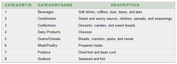
Database used for this demo is: Oracle 10g

Before we begin, we need to understand a few things:

1. Materialized View Log

In an Oracle database, a materialized view log is a table associated with the master table of a materialized view. When master table data undergoes DML changes (such as INSERT, UPDATE, or DELETE), the Oracle database stores rows describing those changes in the materialized view log. A materialized view log is similar to an AUDIT table and is the mechanism used to capture changes made to its related master table. Rows are automatically added to the Materialized View Log table when the master table changes. The Oracle database uses the materialized view log to refresh materialized views based on the master table. This process is called fast refresh and improves performance in the source database.

Ref: Materialized View Log (Oracle Docs)


Table 1: "SS_TIME"

CREATE TABLE "SS_TIME" ("ROW_IDENTIFIER" VARCHAR2(500), "TIME_LEVEL" VARCHAR2(500), "END_DATE" DATE, "TIME_SPAN_IN_DAYS" NUMBER); 

We are going to populate this table using a PL/SQL script.

DECLARE
  start_year number;
  end_year number;
  no_of_days_in_year number;
  date_temp date;
BEGIN
  start_year := 1996;
  end_year := 1997;
  no_of_days_in_year := 365;
  
  /* Inserting rows with level 'year' */
  /*
  FOR i IN start_year .. end_year LOOP
    no_of_days_in_year := MOD(i, 4);
    IF  no_of_days_in_year = 0 THEN
      no_of_days_in_year := 366;
    ELSE
      no_of_days_in_year := 365;
    END IF;
    insert into ss_time values(i, 'YEAR', add_months(to_date(start_year || '-JAN-01', 'YYYY-MON-DD'), 12) - 1, no_of_days_in_year);
  END LOOP;
  */
  
  /* Inserting rows with level 'MONTH' */ 
  FOR i IN start_year .. end_year LOOP
    FOR j in 0..11 LOOP
      date_temp := add_months(to_date(i || '-JAN-01', 'YYYY-MON-DD'), j) - 1;
      INSERT INTO ss_time VALUES(to_char(date_temp, 'MON') || i, 'MONTH', date_temp, extract(day from last_day(date_temp)));
    END LOOP;
  END LOOP;
END; 

Once we run the above script, we get a data as shown below:



Next, we have following tables:

-- CustomerID	CustomerName	ContactName	Address	City	PostalCode	Country
create table ss_customers (customerid number primary key, customername varchar2(1000), contactname varchar2(1000), address varchar2(1000), city varchar2(1000), postalcode varchar2(1000), country varchar2(1000));

-- OrderID	CustomerID	EmployeeID	OrderDate	ShipperID
create table ss_orders (orderid number primary key, customerid number, employeeid number, orderdate date, shipperid number);

-- ProductID	ProductName	SupplierID	CategoryID	Unit	Price
create table ss_products (productid number primary key, productname varchar2(1000), supplierid number, categoryid number, unit varchar2(1000), price number);

-- CategoryID	CategoryName	Description	
create table ss_categories (categoryid number primary key, categoryname varchar2(1000), description varchar2(1000));

-- OrderDetailID	OrderID	ProductID	Quantity
create table ss_orderdetails (orderdetailid number, orderid number, productid number, quantity number); 

Next, we run insert statements for 'SS_CUSTOMERS' using an SQL file.

The file is "Insert Statements for ss_customers.sql", and has contents:

SET DEFINE OFF;
insert into ss_customers values(1, 'Alfreds Futterkiste', 'Maria Anders', 'Obere Str. 57', 'Berlin', '12209', 'Germany');
insert into ss_customers values (2,'Ana Trujillo Emparedados y helados','Ana Trujillo','Avda. de la Constitucion 2222','Mexico D.F.','05021','Mexico');
insert into ss_customers values (3,'Antonio Moreno Taqueria','Antonio Moreno','Mataderos 2312','Mexico D.F.','05023','Mexico');
...
commmit; 

This file is ran from Command Prompt as shown below:



You can view the contents of the table in 'SQL Developer' or 'Oracle 10g Apex Application':



Similarly for "ss_orders":



Similarly for 'ss_products':



Similarly for "ss_categories":



Similarly for "ss_orderdetails":



Testing:
  select * from ss_orders;  --GIVES THE NUMBER OF SALES
  select * from ss_customers; --GIVES THE COUNTRY WHERE SALES WERE MADE
  select * from ss_products;
  select * from ss_categories;
  select * from ss_time;
  select * from ss_orderdetails;
  select decode(sum(customerid),null,0,sum(customerid)) as cust_count from ss_customers where city='Delhi'; 
  
Our OLAP Star Schema will have:
THREE DIMENSIONS: TIME, PRODUCT CATEGORIES (SINGLE VALUED DIMENSION), COUNTRY (SINGLE VALUED DIMENSION)
AND ONE MEASURE: NUMBER OF ORDERS 

Query:

select tim.row_identifier as time_interval, cust.country, cat.categoryname, count(ord.orderid)
  from ss_time tim, ss_customers cust, ss_categories cat, ss_orders ord, ss_orderdetails odd, ss_products prd
  where ord.customerid = cust.customerid
    and odd.productid = prd.productid
    and prd.categoryid = cat.categoryid
    and tim.end_date >= ord.orderdate
    and (tim.end_date - tim.time_span_in_days + 1) <= ord.orderdate
  group by tim.row_identifier, cust.country, cat.categoryname; 
  
OUTPUT:

  

Another Test Query:
select tim.row_identifier as time_interval, ord.orderid
  from ss_time tim, ss_orders ord
  where tim.end_date >= ord.orderdate
    and (tim.end_date - tim.time_span_in_days + 1) <= ord.orderdate; 
	
Next, we create "Materialized View Log(s)":

CREATE MATERIALIZED VIEW LOG ON SS_PRODUCTS
  WITH PRIMARY KEY, ROWID (categoryid)
  INCLUDING NEW VALUES;

CREATE MATERIALIZED VIEW LOG ON SS_ORDERDETAILS
  WITH ROWID (productid)
  INCLUDING NEW VALUES; 
/* The CREATE MATERIALIZED VIEW LOG command was issued with the WITH PRIMARY KEY option and the master table did not contain a primary key constraint or the constraint was disabled. Reissue the command using only the WITH ROWID option, create a primary key constraint on the master table, or enable an existing primary key constraint. */

CREATE MATERIALIZED VIEW LOG ON SS_ORDERS
  WITH PRIMARY KEY, ROWID (customerid, orderdate)
  INCLUDING NEW VALUES;

CREATE MATERIALIZED VIEW LOG ON SS_CATEGORIES
  WITH PRIMARY KEY, ROWID (categoryname)
  INCLUDING NEW VALUES;

CREATE MATERIALIZED VIEW LOG ON SS_CUSTOMERS
  WITH PRIMARY KEY, ROWID (country)
  INCLUDING NEW VALUES;

CREATE MATERIALIZED VIEW LOG ON SS_TIME
  WITH ROWID (row_identifier, end_date, time_span_in_days)
  INCLUDING NEW VALUES;
-- DROP MATERIALIZED VIEW LOG ON ss_time; 

Next, we create the 'Materialized View':

CREATE MATERIALIZED VIEW ss_mv_total_sales_fact_table
  BUILD IMMEDIATE
  REFRESH FAST ON COMMIT
  ENABLE QUERY REWRITE
  AS
    SELECT tim.row_identifier AS time_interval, cust.country, cat.categoryname, count(ord.orderid) as count_orders
      FROM ss_time tim, ss_customers cust, ss_categories cat, ss_orders ord, ss_orderdetails odd, ss_products prd
      WHERE ord.customerid = cust.customerid
        AND odd.productid = prd.productid
        AND prd.categoryid = cat.categoryid
        AND tim.end_date >= ord.orderdate
        AND (tim.end_date - tim.time_span_in_days + 1) <= ord.orderdate
      GROUP BY tim.row_identifier, cust.country, cat.categoryname; 

Testing:

SELECT * FROM ss_mv_total_sales_fact_table;



SELECT * FROM ss_mv_total_sales_fact_table where country = 'Germany' order by categoryname;



SELECT * FROM ss_mv_total_sales_fact_table where country = 'Germany' and time_interval = '1996'; -- No data found.

SELECT * FROM ss_mv_total_sales_fact_table where country = 'Germany' and time_interval like '%1996%' order by categoryname;



All code files are here: Google Drive

Taking table data from Excel to SQL based database

It is a common usecase when we have receive data in Excel sheet (a .XLS or .XLSX file) and we have to take it to an RDBMS such as Oracle Database or PostGRE SQL database.
One way to do this transfer of data is: we first convert table data into SQL queries and then run those queries in the SQL interface of the database.

This is what our Excel sheet looks like:



In the cell [Row 2, Column 7], we insert the following function call to "CONCATENATE":

=CONCATENATE("insert into employees values(",RC[-6],",'",RC[-5],"','",RC[-4],"',to_date('",RC[-3],"','MM/DD/YYYY'),'",RC[-2],"','",RC[-1],"');") 

This fills our cell [Row 2, Column 7] with an 'INSERT' SQL statement. 

insert into employees values(1 ,'Davolio ','Nancy ',to_date('12/8/1968 ','MM/DD/YYYY'),'EmpID1.pic ','Education includes a BA in psychology from Colorado State University. She also completed (The Art of the Cold Call). Nancy is a member of 'Toastmasters International'. '); 

Copying this in the entire 'column 7' produces the SQL statements we want. 

Before running the INSERT statements, we need to have the table "employees" in our database. The 'CREATE TABLE' statement for the "employees" table is:

create table employees (EmployeeID number(5) primary key, LastName varchar2(80), FirstName varchar2(80), BirthDate date, Photo varchar2(80), Notes varchar2(4000)); 

Writing this 'CREATE TABLE' statement requires that we know the datatypes we want for our columns.

Now we can populate our RDBMS database using the generated 'INSERT' statements.

The Excel file used for this demo can be found here: Google Drive