import numpy as np
import pandas as pd
import matplotlib.pyplot as plt
import seaborn as sns
from tensorflow import keras
#import the Keras layers
from tensorflow.keras.models import Sequential
from tensorflow.keras.layers import Embedding,Dense, Dropout, LSTM, Dropout,Activation
from sklearn.preprocessing import MinMaxScaler
from sklearn.metrics import mean_squared_error
from sklearn.utils import shuffle
# Loading data
data = pd.read_csv('files_input/infy/infy_2000 to 2008.csv')
data.info()
<class 'pandas.core.frame.DataFrame'>
RangeIndex: 2496 entries, 0 to 2495
Data columns (total 15 columns):
# Column Non-Null Count Dtype
--- ------ -------------- -----
0 Symbol 2496 non-null object
1 Series 2496 non-null object
2 Date 2496 non-null object
3 Prev Close 2496 non-null float64
4 Open Price 2496 non-null float64
5 High Price 2496 non-null float64
6 Low Price 2496 non-null float64
7 Last Price 2496 non-null float64
8 Close Price 2496 non-null float64
9 Average Price 2496 non-null float64
10 Total Traded Quantity 2496 non-null int64
11 Turnover 2496 non-null float64
12 No. of Trades 2496 non-null object
13 Deliverable Qty 2496 non-null object
14 % Dly Qt to Traded Qty 2496 non-null object
dtypes: float64(8), int64(1), object(6)
memory usage: 292.6+ KB
data.head()
 # Selecting only Date and Average Price columns
data = data[['Open Price', 'Average Price']]
# Scaling the values in the range of 0 to 1
scaler = MinMaxScaler(feature_range = (0, 1))
scaled_price = scaler.fit_transform(data.loc[:, 'Average Price'].values.reshape(-1, 1))
# Splitting dataset in the ratio of 75:25 for training and test
train_size = int(data.shape[0] * 0.75)
train, test = scaled_price[0:train_size, :], scaled_price[train_size:data.shape[0], :]
print("Number of entries (training set, test set): " + str((len(train), len(test))))
Number of entries (training set, test set): (1872, 624)
def create_dataset(scaled_price, window_size=1):
data_X, data_Y = [], []
for i in range(len(scaled_price) - window_size - 1):
a = scaled_price[i:(i + window_size), 0]
data_X.append(a)
data_Y.append(scaled_price[i + window_size, 0])
return(np.array(data_X), np.array(data_Y))
# Create test and training sets for one-step-ahead regression.
window_size = 3
train_X, train_Y = create_dataset(train, window_size)
test_X, test_Y = create_dataset(test, window_size)
print("Original training data shape:")
print(train_X.shape)
# Reshape the input data into appropriate form for Keras.
train_X = np.reshape(train_X, (train_X.shape[0], 1, train_X.shape[1]))
test_X = np.reshape(test_X, (test_X.shape[0], 1, test_X.shape[1]))
print("New training data shape:")
print(train_X.shape)
Original training data shape:
(1868, 3)
New training data shape:
(1868, 1, 3)
The LSTM architecture here consists of:
One input layer.
One LSTM layer of 4 blocks.
One Dense layer to produce a single output.
MSE as loss function.
# Designing the LSTM model
model = Sequential()
model.add(LSTM(4, input_shape = (1, window_size)))
model.add(Dense(1))
2022-08-30 18:27:28.769044: I tensorflow/core/platform/cpu_feature_guard.cc:193] This TensorFlow binary is optimized with oneAPI Deep Neural Network Library (oneDNN) to use the following CPU instructions in performance-critical operations: SSE4.1 SSE4.2 AVX AVX2 FMA
To enable them in other operations, rebuild TensorFlow with the appropriate compiler flags.
# Compiling the model
model.compile(loss = "mean_squared_error", optimizer = "adam")
# Training the model
model.fit(train_X, train_Y, epochs=10, batch_size=1)
Epoch 1/10
1868/1868 [==============================] - 8s 3ms/step - loss: 0.0053
Epoch 2/10
1868/1868 [==============================] - 5s 3ms/step - loss: 4.7545e-04
Epoch 3/10
1868/1868 [==============================] - 5s 3ms/step - loss: 4.2540e-04
Epoch 4/10
1868/1868 [==============================] - 5s 3ms/step - loss: 3.7605e-04
Epoch 5/10
1868/1868 [==============================] - 5s 3ms/step - loss: 3.4645e-04
Epoch 6/10
1868/1868 [==============================] - 5s 3ms/step - loss: 3.4557e-04
Epoch 7/10
1868/1868 [==============================] - 5s 3ms/step - loss: 3.2880e-04
Epoch 8/10
1868/1868 [==============================] - 5s 3ms/step - loss: 3.2757e-04
Epoch 9/10
1868/1868 [==============================] - 5s 3ms/step - loss: 3.0206e-04
Epoch 10/10
1868/1868 [==============================] - 5s 3ms/step - loss: 3.0305e-04
<keras.callbacks.History at 0x7fc9645e75b0>
def predict_and_score(model, X, Y):
# Make predictions on the original scale of the data.
predicted = scaler.inverse_transform(model.predict(X))
# Prepare Y data to also be on the original scale for interpretability.
orig_data = scaler.inverse_transform([Y])
# Calculate RMSE.
score = np.sqrt(mean_squared_error(orig_data[0], predicted[:, 0]))
return(score, predicted)
rmse_train, train_predict = predict_and_score(model, train_X, train_Y)
rmse_test, test_predict = predict_and_score(model, test_X, test_Y)
print("Training data score: %.2f RMSE" % rmse_train)
print("Test data score: %.2f RMSE" % rmse_test)
59/59 [==============================] - 1s 2ms/step
20/20 [==============================] - 0s 2ms/step
Training data score: 248.61 RMSE
Test data score: 63.50 RMSE
# Create the plot for predicted and the training data.
plt.figure(figsize = (15, 5))
plt.plot(scaler.inverse_transform(scaled_price), label = "True value")
plt.plot(train_predict, label = "Training set prediction")
plt.xlabel("Days")
plt.ylabel("Average Price")
plt.title("Comparison true vs. predicted training set")
plt.legend()
plt.show()
# Selecting only Date and Average Price columns
data = data[['Open Price', 'Average Price']]
# Scaling the values in the range of 0 to 1
scaler = MinMaxScaler(feature_range = (0, 1))
scaled_price = scaler.fit_transform(data.loc[:, 'Average Price'].values.reshape(-1, 1))
# Splitting dataset in the ratio of 75:25 for training and test
train_size = int(data.shape[0] * 0.75)
train, test = scaled_price[0:train_size, :], scaled_price[train_size:data.shape[0], :]
print("Number of entries (training set, test set): " + str((len(train), len(test))))
Number of entries (training set, test set): (1872, 624)
def create_dataset(scaled_price, window_size=1):
data_X, data_Y = [], []
for i in range(len(scaled_price) - window_size - 1):
a = scaled_price[i:(i + window_size), 0]
data_X.append(a)
data_Y.append(scaled_price[i + window_size, 0])
return(np.array(data_X), np.array(data_Y))
# Create test and training sets for one-step-ahead regression.
window_size = 3
train_X, train_Y = create_dataset(train, window_size)
test_X, test_Y = create_dataset(test, window_size)
print("Original training data shape:")
print(train_X.shape)
# Reshape the input data into appropriate form for Keras.
train_X = np.reshape(train_X, (train_X.shape[0], 1, train_X.shape[1]))
test_X = np.reshape(test_X, (test_X.shape[0], 1, test_X.shape[1]))
print("New training data shape:")
print(train_X.shape)
Original training data shape:
(1868, 3)
New training data shape:
(1868, 1, 3)
The LSTM architecture here consists of:
One input layer.
One LSTM layer of 4 blocks.
One Dense layer to produce a single output.
MSE as loss function.
# Designing the LSTM model
model = Sequential()
model.add(LSTM(4, input_shape = (1, window_size)))
model.add(Dense(1))
2022-08-30 18:27:28.769044: I tensorflow/core/platform/cpu_feature_guard.cc:193] This TensorFlow binary is optimized with oneAPI Deep Neural Network Library (oneDNN) to use the following CPU instructions in performance-critical operations: SSE4.1 SSE4.2 AVX AVX2 FMA
To enable them in other operations, rebuild TensorFlow with the appropriate compiler flags.
# Compiling the model
model.compile(loss = "mean_squared_error", optimizer = "adam")
# Training the model
model.fit(train_X, train_Y, epochs=10, batch_size=1)
Epoch 1/10
1868/1868 [==============================] - 8s 3ms/step - loss: 0.0053
Epoch 2/10
1868/1868 [==============================] - 5s 3ms/step - loss: 4.7545e-04
Epoch 3/10
1868/1868 [==============================] - 5s 3ms/step - loss: 4.2540e-04
Epoch 4/10
1868/1868 [==============================] - 5s 3ms/step - loss: 3.7605e-04
Epoch 5/10
1868/1868 [==============================] - 5s 3ms/step - loss: 3.4645e-04
Epoch 6/10
1868/1868 [==============================] - 5s 3ms/step - loss: 3.4557e-04
Epoch 7/10
1868/1868 [==============================] - 5s 3ms/step - loss: 3.2880e-04
Epoch 8/10
1868/1868 [==============================] - 5s 3ms/step - loss: 3.2757e-04
Epoch 9/10
1868/1868 [==============================] - 5s 3ms/step - loss: 3.0206e-04
Epoch 10/10
1868/1868 [==============================] - 5s 3ms/step - loss: 3.0305e-04
<keras.callbacks.History at 0x7fc9645e75b0>
def predict_and_score(model, X, Y):
# Make predictions on the original scale of the data.
predicted = scaler.inverse_transform(model.predict(X))
# Prepare Y data to also be on the original scale for interpretability.
orig_data = scaler.inverse_transform([Y])
# Calculate RMSE.
score = np.sqrt(mean_squared_error(orig_data[0], predicted[:, 0]))
return(score, predicted)
rmse_train, train_predict = predict_and_score(model, train_X, train_Y)
rmse_test, test_predict = predict_and_score(model, test_X, test_Y)
print("Training data score: %.2f RMSE" % rmse_train)
print("Test data score: %.2f RMSE" % rmse_test)
59/59 [==============================] - 1s 2ms/step
20/20 [==============================] - 0s 2ms/step
Training data score: 248.61 RMSE
Test data score: 63.50 RMSE
# Create the plot for predicted and the training data.
plt.figure(figsize = (15, 5))
plt.plot(scaler.inverse_transform(scaled_price), label = "True value")
plt.plot(train_predict, label = "Training set prediction")
plt.xlabel("Days")
plt.ylabel("Average Price")
plt.title("Comparison true vs. predicted training set")
plt.legend()
plt.show()
 test_predict_padded = np.concatenate(([[1900], [1900], [1900], [1900]], test_predict))
print("test_predict_padded.shape: ", test_predict_padded.shape)
test_predict_padded.shape: (624, 1)
test_orig = data[['Average Price']].iloc[train_size:data.shape[0], :]
test_orig.reset_index(inplace = True, drop=True)
print("test_orig.shape: ", test_orig.shape)
print("test_predict.shape: ", test_predict.shape)
test_orig.shape: (624, 1)
test_predict.shape: (620, 1)
# Create the plot for predicted and the training data.
plt.figure(figsize = (15, 5))
plt.plot(test_predict_padded[0:200], label = "Test set prediction")
plt.plot(test_orig[0:200], label = "Test set actual data points")
plt.xlabel("Days")
plt.ylabel("Average Price")
plt.title("Comparison true vs. predicted on test set")
plt.legend()
plt.show()
test_predict_padded = np.concatenate(([[1900], [1900], [1900], [1900]], test_predict))
print("test_predict_padded.shape: ", test_predict_padded.shape)
test_predict_padded.shape: (624, 1)
test_orig = data[['Average Price']].iloc[train_size:data.shape[0], :]
test_orig.reset_index(inplace = True, drop=True)
print("test_orig.shape: ", test_orig.shape)
print("test_predict.shape: ", test_predict.shape)
test_orig.shape: (624, 1)
test_predict.shape: (620, 1)
# Create the plot for predicted and the training data.
plt.figure(figsize = (15, 5))
plt.plot(test_predict_padded[0:200], label = "Test set prediction")
plt.plot(test_orig[0:200], label = "Test set actual data points")
plt.xlabel("Days")
plt.ylabel("Average Price")
plt.title("Comparison true vs. predicted on test set")
plt.legend()
plt.show()

Tuesday, August 30, 2022
Prediction of Infy Stock Market Price using LSTM based model
Download Code and Data


Sunday, August 28, 2022
Prediction of Infy stock market price using Recurrent Neural Network
Download Code and Data
This code demonstrates the prediction of stock market price using Recurrent Neural Networks.
Dataset: Infosys stock market price from 2000 to 2008 is used to train the RNN model.
import numpy as np
import pandas as pd
import matplotlib.pyplot as plt
import seaborn as sns
from tensorflow import keras
#import the Keras layers
from tensorflow.keras.models import Sequential
from tensorflow.keras.layers import Embedding,Dense, Dropout, LSTM, Dropout,Activation
from sklearn.preprocessing import MinMaxScaler
from sklearn.metrics import mean_squared_error
from sklearn.utils import shuffle
# Loading data
data = pd.read_csv('files_input/infy/infy_2000 to 2008.csv')
data.info()
<class 'pandas.core.frame.DataFrame'>
RangeIndex: 2496 entries, 0 to 2495
Data columns (total 15 columns):
# Column Non-Null Count Dtype
--- ------ -------------- -----
0 Symbol 2496 non-null object
1 Series 2496 non-null object
2 Date 2496 non-null object
3 Prev Close 2496 non-null float64
4 Open Price 2496 non-null float64
5 High Price 2496 non-null float64
6 Low Price 2496 non-null float64
7 Last Price 2496 non-null float64
8 Close Price 2496 non-null float64
9 Average Price 2496 non-null float64
10 Total Traded Quantity 2496 non-null int64
11 Turnover 2496 non-null float64
12 No. of Trades 2496 non-null object
13 Deliverable Qty 2496 non-null object
14 % Dly Qt to Traded Qty 2496 non-null object
dtypes: float64(8), int64(1), object(6)
memory usage: 292.6+ KB
data.head()
 # Selecting only Date and Average Price columns
data = data[['Open Price', 'Average Price']]
# Scaling the values in the range of 0 to 1
scaler = MinMaxScaler(feature_range = (0, 1))
scaled_price = scaler.fit_transform(data.loc[:, 'Average Price'].values.reshape(-1, 1))
# Splitting dataset in the ratio of 75:25 for training and test
train_size = int(data.shape[0] * 0.75)
train, test = scaled_price[0:train_size, :], scaled_price[train_size:data.shape[0], :]
print("Number of entries (training set, test set): " + str((len(train), len(test))))
Number of entries (training set, test set): (1872, 624)
def create_dataset(scaled_price, window_size=1):
data_X, data_Y = [], []
for i in range(len(scaled_price) - window_size - 1):
a = scaled_price[i:(i + window_size), 0]
data_X.append(a)
data_Y.append(scaled_price[i + window_size, 0])
return(np.array(data_X), np.array(data_Y))
# Create test and training sets for one-step-ahead regression.
window_size = 3
train_X, train_Y = create_dataset(train, window_size)
test_X, test_Y = create_dataset(test, window_size)
print("Original training data shape:")
print(train_X.shape)
# Reshape the input data into appropriate form for Keras.
train_X = np.reshape(train_X, (train_X.shape[0], 1, train_X.shape[1]))
test_X = np.reshape(test_X, (test_X.shape[0], 1, test_X.shape[1]))
print("New training data shape:")
print(train_X.shape)
Original training data shape:
(1868, 3)
New training data shape:
(1868, 1, 3)
Keras simple RNN is layer is built as the first layer, then 2 dense layers is added.
import tensorflow as tf
model = tf.keras.Sequential([
tf.keras.layers.SimpleRNN(32),
tf.keras.layers.Dense(10, activation='relu'),
tf.keras.layers.Dense(1, activation='sigmoid')
])
# SimpleRNN model can also be created using Keras simpleRNN class
# Learners can uncomment the below code to create the simpleRNN using Keras
# from tensorflow.keras.models import Model
# from tensorflow.keras.layers import SimpleRNN
# model = Sequential()
# model.add(SimpleRNN(units = 32, return_sequences=False, unroll=True, input_shape=(6, 2)))
# Compiling the model
model.compile(loss = "mean_squared_error", optimizer = "adam")
# Training the model
model.fit(train_X, train_Y, epochs=10, batch_size=1)
Epoch 1/10
1868/1868 [==============================] - 7s 3ms/step - loss: 0.0077
Epoch 2/10
1868/1868 [==============================] - 4s 2ms/step - loss: 6.4751e-04
Epoch 3/10
1868/1868 [==============================] - 4s 2ms/step - loss: 4.6002e-04
Epoch 4/10
1868/1868 [==============================] - 5s 2ms/step - loss: 4.2450e-04
Epoch 5/10
1868/1868 [==============================] - 5s 2ms/step - loss: 3.8224e-04
Epoch 6/10
1868/1868 [==============================] - 4s 2ms/step - loss: 3.8648e-04
Epoch 7/10
1868/1868 [==============================] - 4s 2ms/step - loss: 3.6662e-04
Epoch 8/10
1868/1868 [==============================] - 4s 2ms/step - loss: 3.8370e-04
Epoch 9/10
1868/1868 [==============================] - 4s 2ms/step - loss: 3.3650e-04
Epoch 10/10
1868/1868 [==============================] - 4s 2ms/step - loss: 3.4760e-04
<keras.callbacks.History at 0x7feaf84d0bb0>
def predict_and_score(model, X, Y):
# Make predictions on the original scale of the data.
predicted = scaler.inverse_transform(model.predict(X))
# Prepare Y data to also be on the original scale for interpretability.
orig_data = scaler.inverse_transform([Y])
# Calculate RMSE.
score = np.sqrt(mean_squared_error(orig_data[0], predicted[:, 0]))
return(score, predicted)
rmse_train, train_predict = predict_and_score(model, train_X, train_Y)
rmse_test, test_predict = predict_and_score(model, test_X, test_Y)
print("Training data score: %.2f RMSE" % rmse_train)
print("Test data score: %.2f RMSE" % rmse_test)
59/59 [==============================] - 1s 2ms/step
20/20 [==============================] - 0s 2ms/step
Training data score: 273.58 RMSE
Test data score: 277.63 RMSE
# Create the plot for predicted and the training data.
plt.figure(figsize = (15, 5))
plt.plot(scaler.inverse_transform(scaled_price), label = "True value")
plt.plot(train_predict, label = "Training set prediction")
plt.xlabel("Days")
plt.ylabel("Average Price")
plt.title("Comparison true vs. predicted training set")
plt.legend()
plt.show()
# Selecting only Date and Average Price columns
data = data[['Open Price', 'Average Price']]
# Scaling the values in the range of 0 to 1
scaler = MinMaxScaler(feature_range = (0, 1))
scaled_price = scaler.fit_transform(data.loc[:, 'Average Price'].values.reshape(-1, 1))
# Splitting dataset in the ratio of 75:25 for training and test
train_size = int(data.shape[0] * 0.75)
train, test = scaled_price[0:train_size, :], scaled_price[train_size:data.shape[0], :]
print("Number of entries (training set, test set): " + str((len(train), len(test))))
Number of entries (training set, test set): (1872, 624)
def create_dataset(scaled_price, window_size=1):
data_X, data_Y = [], []
for i in range(len(scaled_price) - window_size - 1):
a = scaled_price[i:(i + window_size), 0]
data_X.append(a)
data_Y.append(scaled_price[i + window_size, 0])
return(np.array(data_X), np.array(data_Y))
# Create test and training sets for one-step-ahead regression.
window_size = 3
train_X, train_Y = create_dataset(train, window_size)
test_X, test_Y = create_dataset(test, window_size)
print("Original training data shape:")
print(train_X.shape)
# Reshape the input data into appropriate form for Keras.
train_X = np.reshape(train_X, (train_X.shape[0], 1, train_X.shape[1]))
test_X = np.reshape(test_X, (test_X.shape[0], 1, test_X.shape[1]))
print("New training data shape:")
print(train_X.shape)
Original training data shape:
(1868, 3)
New training data shape:
(1868, 1, 3)
Keras simple RNN is layer is built as the first layer, then 2 dense layers is added.
import tensorflow as tf
model = tf.keras.Sequential([
tf.keras.layers.SimpleRNN(32),
tf.keras.layers.Dense(10, activation='relu'),
tf.keras.layers.Dense(1, activation='sigmoid')
])
# SimpleRNN model can also be created using Keras simpleRNN class
# Learners can uncomment the below code to create the simpleRNN using Keras
# from tensorflow.keras.models import Model
# from tensorflow.keras.layers import SimpleRNN
# model = Sequential()
# model.add(SimpleRNN(units = 32, return_sequences=False, unroll=True, input_shape=(6, 2)))
# Compiling the model
model.compile(loss = "mean_squared_error", optimizer = "adam")
# Training the model
model.fit(train_X, train_Y, epochs=10, batch_size=1)
Epoch 1/10
1868/1868 [==============================] - 7s 3ms/step - loss: 0.0077
Epoch 2/10
1868/1868 [==============================] - 4s 2ms/step - loss: 6.4751e-04
Epoch 3/10
1868/1868 [==============================] - 4s 2ms/step - loss: 4.6002e-04
Epoch 4/10
1868/1868 [==============================] - 5s 2ms/step - loss: 4.2450e-04
Epoch 5/10
1868/1868 [==============================] - 5s 2ms/step - loss: 3.8224e-04
Epoch 6/10
1868/1868 [==============================] - 4s 2ms/step - loss: 3.8648e-04
Epoch 7/10
1868/1868 [==============================] - 4s 2ms/step - loss: 3.6662e-04
Epoch 8/10
1868/1868 [==============================] - 4s 2ms/step - loss: 3.8370e-04
Epoch 9/10
1868/1868 [==============================] - 4s 2ms/step - loss: 3.3650e-04
Epoch 10/10
1868/1868 [==============================] - 4s 2ms/step - loss: 3.4760e-04
<keras.callbacks.History at 0x7feaf84d0bb0>
def predict_and_score(model, X, Y):
# Make predictions on the original scale of the data.
predicted = scaler.inverse_transform(model.predict(X))
# Prepare Y data to also be on the original scale for interpretability.
orig_data = scaler.inverse_transform([Y])
# Calculate RMSE.
score = np.sqrt(mean_squared_error(orig_data[0], predicted[:, 0]))
return(score, predicted)
rmse_train, train_predict = predict_and_score(model, train_X, train_Y)
rmse_test, test_predict = predict_and_score(model, test_X, test_Y)
print("Training data score: %.2f RMSE" % rmse_train)
print("Test data score: %.2f RMSE" % rmse_test)
59/59 [==============================] - 1s 2ms/step
20/20 [==============================] - 0s 2ms/step
Training data score: 273.58 RMSE
Test data score: 277.63 RMSE
# Create the plot for predicted and the training data.
plt.figure(figsize = (15, 5))
plt.plot(scaler.inverse_transform(scaled_price), label = "True value")
plt.plot(train_predict, label = "Training set prediction")
plt.xlabel("Days")
plt.ylabel("Average Price")
plt.title("Comparison true vs. predicted training set")
plt.legend()
plt.show()
 test_predict.shape
(620, 1)
test_orig = data[['Average Price']].iloc[train_size:data.shape[0], :]
test_orig.reset_index(inplace = True, drop=True)
print(test_orig.shape)
(624, 1)
test_orig.head()
test_predict.shape
(620, 1)
test_orig = data[['Average Price']].iloc[train_size:data.shape[0], :]
test_orig.reset_index(inplace = True, drop=True)
print(test_orig.shape)
(624, 1)
test_orig.head()
 # Create the plot for predicted and the training data.
plt.figure(figsize = (15, 5))
plt.plot(test_predict, label = "Test set prediction")
plt.plot(test_orig, label = "Test set actual data points")
plt.xlabel("Days")
plt.ylabel("Average Price")
plt.title("Comparison true vs. predicted on test set")
plt.legend()
plt.show()
# Create the plot for predicted and the training data.
plt.figure(figsize = (15, 5))
plt.plot(test_predict, label = "Test set prediction")
plt.plot(test_orig, label = "Test set actual data points")
plt.xlabel("Days")
plt.ylabel("Average Price")
plt.title("Comparison true vs. predicted on test set")
plt.legend()
plt.show()


Thursday, August 25, 2022
A Dynamic Strategy Coach for Effective Negotiation (a Natural Language Processing application) 2019-Sep-30
Download Research Paper
Abstract
Negotiation is a complex activity involving strategic reasoning, persuasion, and psychology. An average person is often far from an expert in negotiation. Our goal is to assist humans to become better negotiators through a machine-in-the-loop approach that combines machine’s advantage at data-driven decisionmaking and human’s language generation ability. We consider a bargaining scenario where a seller and a buyer negotiate the price of an item for sale through a text-based dialog. Our negotiation coach monitors messages between them and recommends tactics in real time to the seller to get a better deal (e.g., “reject the proposal and propose a price”, “talk about your personal experience with the product”). The best strategy and tactics largely depend on the context (e.g., the current price, the buyer’s attitude). Therefore, we first identify a set of negotiation tactics, then learn to predict the best strategy and tactics in a given dialog context from a set of human–human bargaining dialogs. Evaluation on human–human dialogs shows that our coach increases the profits of the seller by almost 60%.1: Introduction
Negotiation is a social activity that requires both strategic reasoning and communication skills (Thompson, 2001; Thompson et al., 2010). Even humans require years of training to become a good negotiator. Past efforts on building automated negotiation agents (Traum et al., 2008; Cuay´ahuitl et al., 2015; Keizer et al., 2017; Cao et al., 2018; Petukhova et al., 2017; Papangelis and Georgila, 2015) has primarily focused on the strategic aspect, where negotiation is formulated as a sequential decision-making process with a discrete action space, leaving aside the rhetorical aspect. Recently, there has been a growing interest in strategic goal-oriented dialog (He et al., 2017; Lewis et al., 2017; Yarats and Lewis, 2018; He et al., 2018) that aims to handle both reasoning and text generation. While the models are good at learning strategies from human–human dialog and selfplay, there is still a huge gap between machine generated text and human utterances in terms of diversity and coherence (Li et al., 2016a,b). In this paper, we introduce a machine-in-theloop approach (cf. Clark et al., 2018) that combines the language skills of humans and the decision-making skills of machines in negotiation dialogs. Our negotiation coach assists users in real time to make good deals in a bargaining scenario between a buyer and a seller. We focus on helping the seller to achieve a better deal by providing suggestions on what to say and how to say it when responding to the buyer at each turn. As shown in Figure 1, during the (human–human) conversation, our coach analyzes the current dialog history, and makes both high-level strategic suggestions (e.g., hpropose a pricei) and low-level rhetoric suggestions (e.g., huse hedge wordsi). The seller then relies on these suggestions to formulate their response. While there exists a huge body of literature on negotiation in behavioral economics (Pruitt, 1981; Bazerman et al., 2000; Fisher and Ury, 1981; Lax and Sebenius, 2006; Thompson et al., 2010), these studies typically provide case studies and generic principles such as “focus on mutual gain”. Instead of using these abstract, static principles, we draw insights from prior negotiation literature and define actionable strategies and tactics conditioned on the negotiation scenario and the dialog context. We take a data-driven approach (§2) using human – human negotiation dialogs collected in a simulated online bargaining setting (He et al., 2018).Figure 1: Our negotiation coach monitors the conversation between the seller and the buyer, and provides suggestions of negotiation tactics to the seller in each turn dynamically, depending on the negotiation scenario, the dialog context, and examples of previous similar dialogs. First, we build detectors to extract negotiation tactics grounded in each turn, such as product embellishment (“The TV works like a champ!”) and side offers (“I can deliver it to you.”) (§3.1). These turn-level tactics allow us to dynamically predict the tactics used in a next utterance given the dialog context. To quantify the effectiveness of each tactic, we further build an outcome predictor to predict the final deal given past tactics sequence extracted from the dialog history (§5). At test time, given the dialog history in each turn, our coach (1) predicts possible tactics in the next turn (§4); (2) uses the outcome predictor to select tactics that will lead to a good deal; (3) retrieves (lexicalized) examples exhibiting the selected tactics and displays them to the seller (§6). To evaluate the effectiveness of our negotiation coach, we integrate it into He et al.’s (2018) negotiation dialog chat interface and deploy the system on Amazon Mechanical Turk (AMT) (§7). We compare with two baselines: the default setting (no coaching) and the static coaching setting where a tutorial on effective negotiation strategies and tactics is given to the user upfront. The results show that our dynamic negotiation coach helps sellers increase profits by 59% and achieves the highest agreement rate.2: Problem Statement
We follow the CraigslistBargain setting of He et al. (2018), where a buyer and a seller negotiate the price of an item for sale. The negotiation scenario is based on listings scraped from craigslist.com, including product description, product photos (if available), and the listing price. In addition, the buyer is given a private target price that they aim to achieve. Two AMT workers are randomly paired to play the role of the seller and the buyer. They negotiate through the chat interface shown in Figure 2 in a strict turn-taking manner. They are instructed to negotiate hard for a favorable price. Once an agreement is reached, either party can submit the price and the other chooses to accept or reject the deal; the task is then completed. Our goal is to help the seller achieve a better deal (i.e. higher final price) by providing suggestions on how to respond to the buyer during the conversation. At each seller’s turn, the coach takes the negotiation scenario and the current dialog history as input and predicts the best tactics to use in the next turn to achieve a higher final price. The seller has the freedom to choose whether to use the recommended tactics.3: Approach
We define a set of diverse tactics S from past study on negotiation in behavioral economics, including both high-level dialog acts (e.g., (propose a price), (describe the product) and low-level lexical features (e.g. (use hedge words). Given the negotiation scenario and the dialog history, the coach takes the following steps (Figure 3) to generate suggestions: 1. The tactics detectors map each turn to a set of tactics in S. 2. The tactics predictor predicts the set of possible tactics in the next turn given the dialog history. For example, if the buyer has proposed a price, possible tactics include proposing a counter price, agreeing with the price etc.3. The tactics selector takes the candidate tactics from the tactics predictor and selects those that lead to a better final deal. 4. The tactics realizer converts the selected tactics to instructions and examples in natural language, which are then presented to the seller. We detail each step in the following sections. 3.1 Tactics Detectors We focus on two broad categories of strategies in behavioral research: (i) integrative, or win–win, negotiation, in which negotiators seek to build relationships and reach an agreement benefiting both parties; and (ii) distributive, or win–lose, negotiation, in which negotiators adversarially promote their own interests, exert power, bluff, and demand (Walton and McKersie, 1965). In practice, effective negotiation often involves both types of strategies (Fisher and Ury, 1981; Lax and Sebenius, 2006; Pruitt, 1981; K. et al., 2000, inter alia). Prior work typically focuses on conceptual tactics (e.g., emphasize mutual interest), rather than actionable tactics in a specific negotiation scenario (e.g., politely decline to lower the price, but offer free delivery). Therefore, we develop datadriven ways to operationalize and quantify these abstract principles. In Table 1, we list our actionable tactics motivated by various negotiation principles. To detect these tactics from turns, we use a mix of learned classifiers for turn-level tactics (e.g., propose prices) and regular expression rules for lexical tactics (e.g., use polite words). To create the training set for learning tactic predictors, we randomly selected 200 dialogs and annotated them with tactics. The detectors use the following features: (1) the number of words overlapping with the product description; (2) the METEOR score (Denkowski and Lavie, 2014) of the turn given the product description as reference; (3) the cosine distance between the turn embedding and the product description embedding. For “Address buyer’s concerns”, we additionally include lexical features indicating a question (e.g.,“why”, “how”, “does”) from the immediate previous buyer’s turns. Table 2 summarizes the number pf training examples and prediction accuracies for each learned classifier. For lexical tactics, we have the following rules: • (Do not propose first) Waiting for the buyer’s proposal allows the seller to better estimate the buyer’s target. The detector simply keeps track of who proposes a price first by detecting (propose a price). • (Negotiate side offers) The seller sometimes negotiates side offers, e.g., offering a free gift card or free delivery. To detect this strategy, we match the turn against a set of phrases, e.g., “throw in”, “throwing in”, “deliver”, “delivery”, “pick up”, “pick it up”, “in cash”. • (Use factive verbs) defined in (Hooper, 1975) (e.g. know); • (Use hedge words) defined in (Hyland, 2005) (e.g. could, would); • (Use certainty words) defined in the LIWC dictionary (Tausczik and Pennebaker, 2010). • (Communicate politely) We include several politeness-related negotiation tactics that were identified by Danescu-Table 1: Actionable tactics designed based on negotiation principles. Some of them are detected by learning classifiers on annotated data, and the rest are detected using pattern matching. Niculescu-Mizil et al. (2013) as most informative features. They include: gratitude, greetings, apology, “please” in the beginning of a turn, “please” later on. Keywords matching is used to detect these tactics. • (Build rapport) Deepening self-disclosure, e.g., “My kid really liked this bike, but he outgrew it”, is one strategy for building rapport. We implemented three tactics detectors to identify selfdisclosure. First, we count first-person pronouns (Derlaga and Berg, 1987; Joinson, 2001). Second, we count mentions of family members and friends, respectively (Wang et al., 2016). It is done by matching lexicons from family and friend categories in LIWC. • (Talk informally) It is detected by matching the keywords in the informal language category in LIWC. • (Show dominance) To detect stubbornness (Tan et al., 2016), we measure the average dominance score of all the words from the Warriner et al.’s (2013)’s dominance ratings of 14,000 words. • (Express negative sentiment) We measure both positive and negative sentiment by counting words from positive and negative categories in LIWC.8: Conclusion
This paper presents a dynamic negotiation coach that can make measurably good recommendations to sellers that can increase their profits. It benefits from grounding in strategies and tactics within the negotiation literature and uses natural language processing and machine learning techniques to identify and score the tactics’ likelihood of being successful. We have tested this coach on human–human negotiations and shown that our techniques can substantially increase the profit of negotiators who follow our coach’s recommendations. A key contribution of this study is a new task and a framework of an automated coach-in-theloop that provides on-the-fly autocomplete suggestions to the negotiating parties. This framework can seamlessly be integrated in goal-oriented negotiation dialog systems (Lewis et al., 2017; He et al., 2018), and it also has stand-alone educational and commercial values. For example, our coach can provide language and strategy guidance and help improve negotiation skills of non-expert negotiators. In commercial settings, it has a clear use case of assisting humans in sales and in customer service. An additional important contribution lies in aggregating negotiation strategies from economics and behavioral research, and proposing novel ways to operationalize the strategies using linguistic knowledge and resources.9: Appendix


Wednesday, August 24, 2022
Negotiation Books (Aug 2019)
Download Books


 # 19 - 23
 # 24 - 27
 # 28 - 32
 # 33 - 37
 # 38 - 42
 # 43 - 46
 # 47 - 51

1. Getting to Yes: Negotiating Agreement Without Giving In-Penguin (Roger Fisher, William L. Ury, 2e, 1991)
2. The Negotiation Book (Steve Gates, 2010, Genre: Thesis)
3. Never Split the Difference. Negotiating As If Your Life Depended On It (Chris Voss, 2016)
4. Negotiation Genius: How to Overcome Obstacles and Achieve Brilliant Results at the Bargaining Table and Beyond (Deepak Malhotra, Max Bazerman, 2007)
5. Getting Past No: Negotiating with Difficult People (William Ury, 1993)
6. Bargaining for Advantage: Negotiation Strategies for Reasonable People (G. Richard Shell, 1999)
7. Difficult Conversations (Bruce Patton, Douglas Stone, and Sheila Heen, 1999)
8. Crucial Conversations (Joseph Grenny, Al Switzler, Ron McMillan, 2001)
9. Getting to Yes with Yourself: And Other Worthy Opponents (William Ury, 2015)
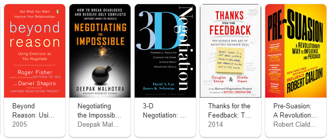
10. Beyond Reasons (Using Emotions as You Negotiate) - Roger Fisher, 2005
11. Negotiating the Impossible (How to break deadlocks and resolve ugly conflicts) - Deepak Malhotra
12. 3-D Negotiation: Powerful Tools to Change the Game in Your Most Important Deals (David Lax and James K. Sebenius)
13. Thanks for the feedback (2014, Douglas Stone and Sheila Heen)
14. Pre-suasion (A revolutionary way to influence and persuade) (Rober Cialdini)
15. Negotiating the Nonnegotiable: How to Resolve Your Most Emotionally Charged Conflicts (Daniel Shapiro)
16. Bargaining with the Devil: When to Negotiate, When to Fight (Robert Harris Mnookin)
17. You Can Negotiate Anything (Herb Cohen)
18. Women Don't Ask (Linda Babcock)
Tuesday, August 23, 2022
Compare two dictionaries in Python
def compare_dict(x, y):
    shared_items = {k: x[k] for k in x if k in y and x[k] == y[k]}
    differing_values = {k: x[k] for k in x if k in y and x[k] != y[k]}
    differing_keys = [k for k in x if k not in y]

    return {
        "shared_items_in_x": shared_items,
        "differing_values_in_x": differing_values,
        "differing_keys_in_x": differing_keys
    }

def is_dict_in_list(d, l):
    rtn = False
    for k in l:
        cd = compare_dict(d, k)
        if(len(cd['differing_values_in_x']) == 0 and len(cd['differing_keys_in_x']) == 0):
            rtn = True
            break
    return rtn

def purify_list_of_dicts(inlist):
    nlist = [i for j in inlist for i in j]

    olist = []

    for i in range(0, len(nlist)):
        if is_dict_in_list(nlist[i], olist) == False:
            olist.append(nlist[i])

    return olist
Thursday, August 11, 2022
Using Sentiment to Detect Bots on Twitter : Are Humans more Opinionated than Bots (Dickerson, Jul 2022)
Download Research Paper
Abstract
In many Twitter applications, developers collect only a limited sample of tweets and a local portion of the Twitter network. Given such Twitter applications with limited data, how can we classify Twitter users as either bots or humans? We develop a collection of network-, linguistic-, and application oriented variables that could be used as possible features, and identify specific features that distinguish well between humans and bots. In particular, by analyzing a large dataset relating to the 2014 Indian election, we show that a number of sentiment related factors are key to the identification of bots, significantly increasing the Area under the ROC Curve (AUROC). The same method may be used for other applications as well.A. Previous Work
There has been recent interest in the detection of malicious and/or fake users from both the online social networks and computer networking communities. # For instance, Wang [4] looks at graph-based features to identify bots on Twitter, while Yang, Harkreader, and [4] A. H. Wang, “Detecting spam bots in online social networking sites: A machine learning approach,” in Conference on Data and Applications Security and Privacy. ACM, 2010, pp. 335–342. # Gu [5] combine similar graphbased features with syntactic metrics to build their classifiers. [5] C. Yang, R. C. Harkreader, and G. Gu, “Die free or live hard? Empirical evaluation and new design for fighting evolving Twitter spammers,” in Recent Advances in Intrusion Detection. Springer, 2011, pp. 318–337. # Thomas et al. [6] use a similar set of features to provide a retrospective analysis of a large set of recently-suspended Twitter accounts. [6] K. Thomas, C. Grier, D. Song, and V. Paxson, “Suspended accounts in retrospect: An analysis of Twitter spam,” in Internet Measurement Conference (IMC). ACM, 2011, pp. 243–258. # Boshmaf et al. [7] instead create bots (rather than detecting them), claiming that 80% of bots are undetectable and that Facebook’s Immune system [8] was unable to detect their bots. [7] Y. Boshmaf, I. Muslukhov, K. Beznosov, and M. Ripeanu, “The socialbot network: When bots socialize for fame and money,” in Annual Computer Security Applications Conference (ACSAC). ACM, 2011, pp. 93–102. [8] T. Stein, E. Chen, and K. Mangla, “Facebook immune system,” in Workshop on Social Network Systems (SNS). ACM, 2011. # Lee, Caverlee, and Webb [9] create “honeypot” accounts to lure both humans and spammers into the open, then provide a statistical analysis of the malicious accounts they identified. [9] K. Lee, J. Caverlee, and S. Webb, “Uncovering social spammers: Social honeypots + machine learning,” in Annual ACM SIGIR Conference on Research and Development in Information Retrieval. ACM, 2010, pp. 435–442. # In computer networks research, the detection of Sybil accounts in computer networks has been applied to social network data; these techniques tend to rely on the “fast mixing” property of a network—which may not exist in social networks [10]—and do not scale to the size of present-day social networks (e.g., SybilInfer [3] runs in time O(|V|^2 . log |V|), which is intractable for networks with millions users). [10] A. Mohaisen, A. Yun, and Y. Kim, “Measuring the mixing time of social graphs,” in Internet Measurement Conference (IMC). ACM, 2010, pp. 383–389.V. CONCLUSION
In many real-world applications, developers are only able to collect tweets from the Twitter API that directly address a set of topics of interest (TOI) relevant to the application. Moreover, in such applications, developers also typically only collect a local portion of the Twitter network. As a consequence, many traditional primarily network-based methods for detecting bots are less or not effective (e.g., if the topics are quite specific, not discussed by very popular people, or not retweeted much), since a sparse subset of the global network and tweet database based on a set TOI is insufficient. The SentiBot framework presented in this paper addresses the classification of users as human versus bot in such applications. In order to achieve this, SentiBot relies on four classes of variables (or features) related to tweet syntax, tweet semantics, user behavior, and network-centric user properties. In particular, we introduce a large set of sentiment variables, including combinations of sentiment and network variables— to our knowledge, this is the first time such sentiment-based features have been used in bot detection. In addition, we introduce variables related to topics of interest. We apply a suite of classical machine learning algorithms to identify: (i) users who are bots and (ii) TOI-independent features that are particularly important in distinguishing between bots and humans. Based on an analysis of over 7.7 million tweets and 550,000 users associated with the recently concluded 2014 Indian election (where there were reports of social media campaigns), we were able to show that the use of sentiment variables significantly improved the accuracy of our classification. In particular, the Area under the ROC Curve (AUROC) increased from 0.65 to 0.73. As an AUROC of 0.5 represents random guessing, this reflects 53% improvement in accuracy. In addition, we discovered that (in our dataset): 1) Bots flip-flop much less frequently than humans in terms of sentiment; 2) When humans express positive sentiment, they tend to express stronger positive sentiment than bots; 3) A similar (but slightly more nuanced) trend holds in terms of expression of negative sentiments by humans; and 4) Humans disagree more with the general sentiment of the application's Twitter population than bots. Our results can feed into many applications. For instance, when assessing which Twitter users are influential on a given topic, we must discount for bots—which requires methods like those presented in this paper to identify bots. When identifying the expected spread of a sentiment through Twitter, we again must discount for bots. The paper presents a general framework within which applications can identify bots using the relatively limited local data they have.
Fluoxetine (SSRI (Selective Serotonin Reuptake Inhibitor))
Fluoxetine, sold under the brand names Prozac and Sarafem, among others, is an antidepressant of the selective serotonin reuptake inhibitor class. It is used for the treatment of major depressive disorder, obsessive–compulsive disorder, bulimia nervosa, panic disorder, and premenstrual dysphoric disorder.Fluoxetine Uses
Fluoxetine is used in the treatment of depression, Panic disorder and obsessive-compulsive disorder.How Fluoxetine works
Fluoxetine is a selective serotonin reuptake inhibitor (SSRI) antidepressant. It works by increasing the levels of serotonin, a chemical messenger in the brain. This improves mood and physical symptoms of depression and also relieves symptoms of panic and obsessive disorders.Common side effects of Fluoxetine
Weakness, Insomnia (difficulty in sleeping), Nervousness, Anxiety, Blurred vision, Decreased libido, Fatigue, Frequent urge to urinate, Gastrointestinal disturbance, Headache, Palpitations, Prolonged QT intervalComposition
Fluoxetine: 20 mg Capsule
Wednesday, August 10, 2022
Classification of Twitter Accounts into Automated Agents and Human Users (Zafar Gilani, Jul 2022)
Download Research Paper
Abstract
Online social networks (OSNs) have seen a remarkable rise in the presence of surreptitious automated accounts. Massive human user-base and business-supportive operating model of social networks (such as Twitter) facilitates the creation of automated agents. In this paper we outline a systematic methodology and train a classifier to categorise Twitter accounts into ‘automated’ and ‘human’ users. To improve classification accuracy we employ a set of novel steps. First, we divide the dataset into four popularity bands to compensate for differences in types of accounts. Second, we create a large ground truth dataset using human annotations and extract relevant features from raw tweets. To judge accuracy of the procedure we calculate agreement among human annotators as well as with a bot detection research tool. We then apply a Random Forests classifier that achieves an accuracy close to human agreement. Finally, as a concluding step we perform tests to measure the efficacy of our results.Index Terms
Social network analysis; account classification; automated agents; bot detectionOur work has the following contributions:
(i) Use of raw historical data (60 million tweets) for attribute collection and account classification (722; 109 tweets) to cater for stealthier agents that are harder to discern from humans; (ii) A Twitter dataset divided into user popularity bands, further partitioned into lists of agents and humans (for reasons refer to xIV) using a human annotation task. This serves as a large ground truth dataset; (iii) 14 novel features from a total feature-set of 21 attributes (see xIV); (iv) Performance evaluation of current state of the art in bot detection by calculating agreement between human annotators and BOTORNOT; (v) Application of supervised learning approach – Random Forests classifier – for non-partisan account categorisation; (vi) Identification of a distinct group of features (using ablation tests) that are most informative for classifying automated agents within each popularity band (cf. Table VIII); and (vii) Hypotheses (cf. Table I) verification against our findings using t-tests (see xVI).Infotainment


References
12: Datasets can be found here – https://goo.gl/SigsQB. Classifier is available as a part of Stweeler. The link is forbidden for public.


Tuesday, August 9, 2022
Accessing Twitter API From Two Systems. One With Firewall and Second Without Firewall
This note is less about accessing Twitter API but more about Cyber Security where you run a curl command and based on the output from that command you try to figure out the firewall settings of the system.

System 1 Configuration With Strict Firewall Where Our Curl Command For Accessing Twitter API is Not Working:

(base) C:\Users\ash\Desktop>systeminfo
OS Name:                   Microsoft Windows 10 Enterprise
OS Version:                10.0.19042 N/A Build 19042

Processor(s):              1 Processor(s) Installed.
                              [01]: AMD64 Family 23 Model 24 Stepping 1 AuthenticAMD ~2100 Mhz
BIOS Version:              HP R79 Ver. 01.10.03, 3/24/2020

Network Card(s):           4 NIC(s) Installed.
                              [01]: Realtek RTL8822BE 802.11ac PCIe Adapter
                                    Connection Name: Wi-Fi
                                    DHCP Enabled:    Yes
                                    DHCP Server:     192.168.1.1
                                    IP address(es)
                                    [01]: 192.168.1.100
                                    [02]: fe80::b1b2:6d59:f669:1b96
                                    [03]: 2401:4900:47f1:b174:70f4:de28:6287:b1c9
                                    [04]: 2401:4900:47f1:b174:b1b2:6d59:f669:1b96
                              [02]: Realtek PCIe GbE Family Controller
                                    Connection Name: Ethernet
                                    Status:          Media disconnected
                              [03]: Bluetooth Device (Personal Area Network)
                                    Connection Name: Bluetooth Network Connection
                                    Status:          Media disconnected
                              [04]: Check Point Virtual Network Adapter For Endpoint VPN Client
                                    Connection Name: Ethernet 2
                                    DHCP Enabled:    Yes
                                    DHCP Server:     10.79.251.145
                                    IP address(es)
                                    [01]: 10.79.251.146
                                    [02]: fe80::3df2:2a4:b2e1:cb0
Hyper-V Requirements:      VM Monitor Mode Extensions: Yes
                              Virtualization Enabled In Firmware: Yes
                              Second Level Address Translation: Yes
                              Data Execution Prevention Available: Yes


System 2 Without Strict Firewall Where Curl Command is Working:


C:\Users\Ashish Jain>systeminfo

Host Name:                 LAPTOP-79RV456R
OS Name:                   Microsoft Windows 10 Home Single Language
OS Version:                10.0.19043 N/A Build 19043
OS Manufacturer:           Microsoft Corporation
OS Configuration:          Standalone Workstation
OS Build Type:             Multiprocessor Free
Registered Owner:          Ashish Jain
Registered Organization:
Product ID:                00327-35105-52167-AAOEM
Original Install Date:     3/14/2021, 6:33:25 AM
System Boot Time:          7/14/2022, 5:34:13 PM
System Manufacturer:       LENOVO
System Model:              81H7
System Type:               x64-based PC
Processor(s):              1 Processor(s) Installed.
                              [01]: Intel64 Family 6 Model 78 Stepping 3 GenuineIntel ~2000 Mhz
BIOS Version:              LENOVO 8QCN26WW(V1.14), 12/29/2020
Windows Directory:         C:\WINDOWS
System Directory:          C:\WINDOWS\system32
Boot Device:               \Device\HarddiskVolume1
System Locale:             en-us;English (United States)
Input Locale:              00004009
Time Zone:                 (UTC+05:30) Chennai, Kolkata, Mumbai, New Delhi
Total Physical Memory:     12,154 MB
Available Physical Memory: 7,634 MB
Virtual Memory: Max Size:  14,010 MB
Virtual Memory: Available: 8,057 MB
Virtual Memory: In Use:    5,953 MB
Page File Location(s):     C:\pagefile.sys
Domain:                    WORKGROUP
Logon Server:              \\LAPTOP-79RV456R
Hotfix(s):                 15 Hotfix(s) Installed.
                              [01]: KB5013887
                              [02]: KB4562830
                              [03]: KB4577586
                              [04]: KB4580325
                              [05]: KB4589212
                              [06]: KB5000736
                              [07]: KB5015807
                              [08]: KB5006753
                              [09]: KB5007273
                              [10]: KB5011352
                              [11]: KB5011651
                              [12]: KB5014032
                              [13]: KB5014035
                              [14]: KB5014671
                              [15]: KB5005699
Network Card(s):           4 NIC(s) Installed.
                              [01]: VirtualBox Host-Only Ethernet Adapter
                                    Connection Name: VirtualBox Host-Only Network
                                    DHCP Enabled:    No
                                    IP address(es)
                                    [01]: 192.168.56.1
                                    [02]: fe80::f839:dc84:9a7b:3087
                              [02]: Realtek 8821CE Wireless LAN 802.11ac PCI-E NIC
                                    Connection Name: Wi-Fi
                                    Status:          Media disconnected
                              [03]: Realtek PCIe FE Family Controller
                                    Connection Name: Ethernet
                                    Status:          Media disconnected
                              [04]: Bluetooth Device (Personal Area Network)
                                    Connection Name: Bluetooth Network Connection
                                    Status:          Media disconnected
Hyper-V Requirements:      VM Monitor Mode Extensions: Yes
                              Virtualization Enabled In Firmware: Yes
                              Second Level Address Translation: Yes
                              Data Execution Prevention Available: Yes

C:\Users\Ashish Jain>


I was able to make a successful request from System 2:


(base) C:\Users\Ashish Jain>curl "https://api.twitter.com/2/users/by/username/vantagepoint21" -H "Authorization: Bearer A***V"

{"data":{"id":"96529689","name":"Ashish Jain","username":"vantagepoint21"}}

(base) C:\Users\Ashish Jain>curl "https://api.twitter.com/2/users/by/username/elonmusk" -H "Authorization: Bearer A***V"

{"data":{"id":"44196397","name":"Elon Musk","username":"elonmusk"}}


The curl command is not working on the System 1.

I think there is some issue being created by Network Firewall settings in my office laptop. From which I was not able to get a response from Twitter API.

(base) C:\Users\ash\Desktop\twitter_api>curl "https://api.twitter.com/2/users/by/username/vantagepoint21" -H "Authorization: Bearer 9***2"

curl: (35) schannel: next InitializeSecurityContext failed: Unknown error (0x80092012) - The revocation function was unable to check revocation for the certificate.

On further testing the "curl" command on 'System 1' for URLs with "http" and "https" protocols:

(base) C:\Users\ash\Desktop>curl www.survival8.blogspot.com
<HTML>
<HEAD>
<TITLE>Moved Permanently</TITLE>
</HEAD>
<BODY BGCOLOR="#FFFFFF" TEXT="#000000">
<H1>Moved Permanently</H1>
The document has moved <A HREF="http://survival8.blogspot.com/">here</A>.
</BODY>
</HTML>

Success for HTTP based URL

---

(base) C:\Users\ash\Desktop>curl https://survival8.blogspot.com
curl: (35) schannel: next InitializeSecurityContext failed: Unknown error (0x80092012) - The revocation function was unable to check revocation for the certificate.

(base) C:\Users\ash\Desktop>curl https://survival8.blogspot.com/2022/08/lets-talk-about-whataboutery.html
curl: (35) schannel: next InitializeSecurityContext failed: Unknown error (0x80092012) - The revocation function was unable to check revocation for the certificate.

Failure for HTTPS based URL.

---

Successful Testing With Another HTTP based URL:

(base) C:\Users\ash\Desktop>curl http://survival8.blogspot.com/2022/08/lets-talk-about-whataboutery.html


<!DOCTYPE html>
<html class='v2' dir='ltr' lang='en'>
<head>
<link href='https://www.blogger.com/static/v1/widgets/2975350028-css_bundle_v2.css' rel='stylesheet' type='text/css'/>
<meta content='width=1100' name='viewport'/>
<meta content='text/html; charset=UTF-8' http-equiv='Content-Type'/>
<meta content='blogger' name='generator'/>
<link href='http://survival8.blogspot.com/favicon.ico' rel='icon' type='image/x-icon'/>
<link href='http://survival8.blogspot.com/2022/08/lets-talk-about-whataboutery.html' rel='canonical'/>
<link rel="alternate" type="application/atom+xml" title="survival8 - Atom" href="http://survival8.blogspot.com/feeds/posts/default" />
<link rel="alternate" type="application/rss+xml" title="survival8 - RSS" href="http://survival8.blogspot.com/feeds/posts/default?alt=rss" />
<link rel="service.post" type="application/atom+xml" title="survival8 - Atom" href="https://draft.blogger.com/feeds/7823701911930369175/posts/default" />

<link rel="alternate" type="application/atom+xml" title="survival8 - Atom" href="http://survival8.blogspot.com/feeds/1169952638388485943/comments/default" />
<!--Can't find substitution for tag [blog.ieCssRetrofitLinks]-->
<meta content='http://survival8.blogspot.com/2022/08/lets-talk-about-whataboutery.html' property='og:url'/>
<meta content='Let’s talk about ‘Whataboutery’' property='og:title'/>
<meta content='                                 what·about·ery [ˌwɒtəˈbaʊtəri] NOUN BRITISH the technique or practice of responding to an accusation or dif...' property='og:description'/>
<title>survival8: Let’s talk about ‘Whataboutery’</title>
<style id='page-skin-1' type='text/css'><!--
/*
-----------------------------------------------
Blogger Template Style
Name:     Simple
Designer: Blogger
URL:      www.blogger.com
----------------------------------------------- */
/* Content
----------------------------------------------- */
body { ...


Also, note that if that was Authorization failure from Twitter API, then the output would still be a JSON format informative message:

(base) C:\Users\Ashish Jain>curl "https://api.twitter.com/2/users/by/username/elonmusk" -H "Authorization: Bearer 9***INCORRECT_BEARER_TOKEN***2"


{
  "title": "Unauthorized",
  "type": "about:blank",
  "status": 401,
  "detail": "Unauthorized"
}


On a Side Note: Take a look at another error message from Twitter API:

(base) C:\Users\Ashish Jain>curl "https://api.twitter.com/2/users/by/username/elonmusj" -H "Authorization: Bearer A***V"


{  "errors":
      [
        {
          "parameter":"username",
          "resource_id":"elonmusj",
          "value":"elonmusj",
          "detail":"User has been suspended: [elonmusj].",
          "title":"Forbidden",
          "resource_type":"user",
          "type":"https://api.twitter.com/2/problems/resource-not-found"
        }
      ]
}


Notice the typo in Elon Musk's user handle we provided in query: elonmusj
Sunday, August 7, 2022
Diclogem Tablet (Diclofenac (50mg) + Paracetamol (325mg))
Diclogem Tablet Prescription Required Manufacturer: Omega Pharmaceuticals Pvt Ltd SALT COMPOSITION: Diclofenac (50mg) + Paracetamol (325mg) Storage: Store below 30°CProduct introduction
Diclogem Tablet is a pain-relieving medicine. It is used to reduce pain and inflammation in conditions like rheumatoid arthritis, ankylosing spondylitis, and osteoarthritis. It may also be used to relieve muscle pain, back pain, toothache, or pain in the ear and throat. Diclogem Tablet should be taken with food. This will prevent you from getting an upset stomach. You should take it regularly as advised by your doctor. Do not take more or use it for a longer duration than recommended by your doctor. Some of the common side effects of this medicine include nausea, vomiting, stomach pain, loss of appetite, heartburn, and diarrhea. If any of these side effects bother you or do not go away with time, you should let your doctor know. Your doctor may help you with ways to reduce or prevent the side effects. The medicine may not be suitable for everybody. Before taking it, let your doctor know if you have any problems with your heart, kidneys, liver, or have stomach ulcers. To make sure it is safe for you, let your doctor know about all the other medicines you are taking. Pregnant and breastfeeding mothers should first consult their doctors before using this medicine.Uses of Diclogem Tablet
Pain reliefBenefits of Diclogem Tablet
In Pain relief Diclogem Tablet is a combination of medicines that is used for short-term relief of pain, inflammation and swelling. It inhibits release of those chemical messengers in the brain that tell us that we have pain. It effectively relieves back pain, earache, throat pain, toothache and pain due to arthritis too. Take it as it is prescribed to get the most benefit. Do not take more or for longer than needed as that can be dangerous. In general, you should take the lowest dose that works, for the shortest possible time. This will help you to go about your daily activities more easily and have a better, more active, quality of life.Side effects of Diclogem Tablet
Most side effects do not require any medical attention and disappear as your body adjusts to the medicine. Consult your doctor if they persist or if you’re worried about them: Common side effects of Diclogem Nausea Vomiting Stomach pain/epigastric pain Heartburn Diarrhea Loss of appetiteFact Box
Habit Forming : No Therapeutic Class : PAIN ANALGESICS
Subscribe to:
Posts (Atom)