survival8: Summary of Support Vector Machines (SVM) - Based on Video by Intuitive Machine Learning

Monday, August 26, 2024

Summary of Support Vector Machines (SVM) - Based on Video by Intuitive Machine Learning

To See All ML Articles: Index of Machine Learning



Support Vector Machines (SVM) are among the top non-linear supervised learning models.

SVMs help identify the optimal hyperplane to categorize data. In one dimension, a hyperplane is a point; in two dimensions, it’s a line; and in three dimensions, it’s a surface that separates positive and negative categories.

Linear Model: For linearly separable data, there are multiple ways to draw a hyperplane that separates positive and negative samples. 



While all hyperplanes separate the categories, SVMs help choose the best one by maximizing the margin, earning them the name “maximum margin classifier.”

What is a support vector? Support vectors are the data points closest to the hyperplane. 



Identifying these crucial data points, whether negative or positive, is a key challenge that SVMs address.

Unlike other models like linear regression or neural networks, where all data points influence the final optimization, in SVMs, only support vectors impact the final decision boundary. When a support vector moves, the decision boundary changes, but moving other vectors has no effect.

Similar to other machine learning models: 



SVMs optimize weights so that only support vectors determine the weights and the decision boundary.

Understanding the mathematical process behind SVMs requires knowledge of linear algebra and optimization theory. Before diving into model calculations, it’s important to understand H0, H1, H2, and W, as shown in the image. W is drawn perpendicular to H0. 



Equation for ( H_0 )



The equation for the hyperplane ( H_0 ) is ( W dot X + b = 0 ). This applies to any number of dimensions. For example, in a two-dimensional scenario, the equation becomes ( W_1 dot X_1 + W_2 dot X_2 + b = y ).

Since ( H_0 ) is defined as ( W dot X + b = 0 ):

( H_1 ) is ( W dot X + b \geq 0 ), which can be rewritten as ( W dot X + b = k ), where ( k ) is a variable. For easier mathematical calculations, we set ( k = 1 ), so ( W dot X + b = 1 ).
( H_2 ) is ( W dot X + b < 0 ), which can be rewritten as ( W dot X + b = -k ). Again, setting ( k = 1 ), we get ( W dot X + b = -1 ).

Applying Lagrange Multipliers

Lagrange Multipliers help identify local maxima and minima subject to equality constraints, forming the decision rule. The assumption here is that the data is linearly separable with no outliers, known as Hard Margin SVM. 



Handling Noise and Outliers

If the data contains noise or outliers, Hard Margin SVM fails to optimize. To address this, Soft Margin SVM is used.

By adding “theta” as constraints to the optimization problem, it becomes possible to satisfy constraints even if outliers do not meet the original constraints. However, this requires a large volume of data where all examples satisfy the constraints.

Regularization:

One technique to handle this problem is Regularization. L1 regularization can be used to penalize large values of theta, with a constant “C” as the regularization parameter. If ( C ) is small, theta is significant; otherwise, it is less important.

Setting ( C ) to a positive infinite value results in the same output as Hard Margin SVM.
A smaller ( C ) value results in a wider margin, while a larger ( C ) value results in a narrower margin. A narrow margin is less tolerant to outliers.
This way, Soft Margin SVM can handle non-linearly separable data with outliers and noise.

Kernel Trick

When data is inherently non-linearly separable, as shown in the example below, the solution is to use the kernel trick. 



The kernel trick introduces a variable ( k ) that squares ( x ), helping to solve the problem. This approach is derived from applying the Lagrange equation. By squaring ( x ), we can achieve a clear separation of the data, allowing us to draw a separating line. 



Polynomial Kernel

This kernel uses two parameters: a constant ( C ) and the degree of freedom ( d ). A larger ( d ) value makes the boundary more complex, which might result in overfitting. 



RBF Kernel (Gaussian Kernel)

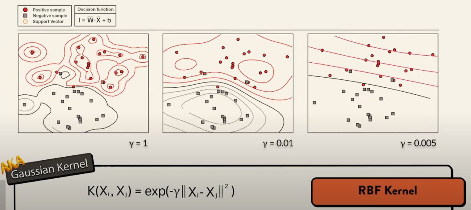
The RBF kernel has one parameter, ( gamma ). A smaller ( gamma ) value leads to a linear SVM, while a larger value heavily impacts the support vectors and may result in overfitting.