Installation of Elephas (for distributed deep learning) on Ubuntu through archives (Apr 2020)

Elephas is an extension of Keras, which allows you to run distributed deep learning models at scale with Spark. Elephas currently supports a number of applications, including:

% Data-parallel training of deep learning models
% Distributed hyper-parameter optimization
% Distributed training of ensemble models

Schematically, elephas works as follows.


We have listed packages that are required outside of Anaconda distribution.
The following code goes in a Shell (.sh) script for Ubuntu or .bat script Windows:
pip install Keras_Applications-1.0.8.tar.gz
pip install keras-team-keras-preprocessing-1.1.0-0-gff90696.tar.gz
pip install Keras-2.3.1.tar.gz
pip install hyperopt-0.2.4-py2.py3-none-any.whl
pip install hyperas-0.4.1-py3-none-any.whl
pip install tensorflow_estimator-2.1.0-py2.py3-none-any.whl 
pip install grpcio-1.28.1-cp37-cp37m-manylinux2010_x86_64.whl
pip install protobuf-3.11.3-cp37-cp37m-manylinux1_x86_64.whl
pip install gast-0.3.3.tar.gz
pip install opt_einsum-3.2.1.tar.gz
pip install astor-0.8.1.tar.gz
pip install absl-py-0.9.0.tar.gz
pip install cachetools-4.1.0.tar.gz
pip install pyasn1-0.4.8.tar.gz
pip install pyasn1-modules-0.2.8.tar.gz
pip install rsa-4.0.tar.gz
pip install google-auth-1.14.1.tar.gz
pip install oauthlib-3.1.0.tar.gz
pip install requests-oauthlib-1.3.0.tar.gz
pip install google-auth-oauthlib-0.4.1.tar.gz
pip install Markdown-3.2.1.tar.gz
pip install tensorboard-2.1.1-py3-none-any.whl
pip install google-pasta-0.2.0.tar.gz
pip install gast-0.2.2.tar.gz
pip install termcolor-1.1.0.tar.gz
pip install tensorflow-2.1.0-cp37-cp37m-manylinux2010_x86_64.whl
pip install pypandoc-1.5.tar.gz
pip install py4j-0.10.7.zip
pip install pyspark-2.4.5.tar.gz
pip install elephas-0.4.3-py3-none-any.whl 

Generated .whl files are stored in directory (here 'ashish' is my username): /home/ashish/.cache/pip/wheels

Few packages were not accepted for latest release labels:
# tensorflow-estimator [2.2.0, >=2.1.0rc0] (from tensorflow==2.1.0). Latest available is: 2.2.0
# pip install gast-0.3.3.tar.gz
# pip install py4j-0.10.9.tar.gz

Most of these packages are required by TensorFlow, except:
1. hyperopt-0.2.4-py2.py3-none-any.whl
2. hyperas-0.4.1-py3-none-any.whl
3. pypandoc-1.5.tar.gz
4. py4j-0.10.7.zip
5. pyspark-2.4.5.tar.gz

All the packages are present in this Google Drive link, except TensorFlow and PySpark due to their sizes.
PySpark size: 207 MB
TensorFlow size: 402 MB

Running the shell script second time, uninstalls and reinstalls the packages again.
Here is a Python script to avoid doing this and install only if packages are not installed already:

import sys
import subprocess
import pkg_resources

required = { 'pyspark', 'scipy', 'tensorflow' }
installed = { pkg.key for pkg in pkg_resources.working_set }
missing = required - installed

if missing:
    python = sys.executable
    subprocess.check_call([python, '-m', 'pip', 'install', *missing], stdout=subprocess.DEVNULL) 

References:
1. Elephas Documentation
2. GitHub Repository

Tags: Technology,Deep Learning,Machine Learning,Big Data,

Prediction of Infy Stock Market Price using LSTM based model

Download Code and Data

import numpy as np
import pandas as pd
import matplotlib.pyplot as plt
import seaborn as sns
from tensorflow import keras
#import the Keras layers
from tensorflow.keras.models import Sequential
from tensorflow.keras.layers import Embedding,Dense, Dropout, LSTM, Dropout,Activation
from sklearn.preprocessing import MinMaxScaler
from sklearn.metrics import mean_squared_error
from sklearn.utils import shuffle 

# Loading data
data = pd.read_csv('files_input/infy/infy_2000 to 2008.csv')
data.info() 


<class 'pandas.core.frame.DataFrame'>
RangeIndex: 2496 entries, 0 to 2495
Data columns (total 15 columns):
    #   Column                  Non-Null Count  Dtype  
   ---  ------                  --------------  -----  
    0   Symbol                  2496 non-null   object 
    1   Series                  2496 non-null   object 
    2   Date                    2496 non-null   object 
    3   Prev Close              2496 non-null   float64
    4   Open Price              2496 non-null   float64
    5   High Price              2496 non-null   float64
    6   Low Price               2496 non-null   float64
    7   Last Price              2496 non-null   float64
    8   Close Price             2496 non-null   float64
    9   Average Price           2496 non-null   float64
    10  Total Traded Quantity   2496 non-null   int64  
    11  Turnover                2496 non-null   float64
    12  No. of Trades           2496 non-null   object 
    13  Deliverable Qty         2496 non-null   object 
    14  % Dly Qt to Traded Qty  2496 non-null   object 
dtypes: float64(8), int64(1), object(6)
memory usage: 292.6+ KB     



data.head()





# Selecting only Date and Average Price columns
data = data[['Open Price', 'Average Price']]

# Scaling the values in the range of 0 to 1
scaler = MinMaxScaler(feature_range = (0, 1))
scaled_price = scaler.fit_transform(data.loc[:, 'Average Price'].values.reshape(-1, 1))

# Splitting dataset in the ratio of 75:25 for training and test
train_size = int(data.shape[0] * 0.75)
train, test = scaled_price[0:train_size, :], scaled_price[train_size:data.shape[0], :]
print("Number of entries (training set, test set): " + str((len(train), len(test))))


Number of entries (training set, test set): (1872, 624)


def create_dataset(scaled_price, window_size=1):
    data_X, data_Y = [], []
    for i in range(len(scaled_price) - window_size - 1):
        a = scaled_price[i:(i + window_size), 0]
        data_X.append(a)
        data_Y.append(scaled_price[i + window_size, 0])
    return(np.array(data_X), np.array(data_Y))

# Create test and training sets for one-step-ahead regression.
window_size = 3
train_X, train_Y = create_dataset(train, window_size)
test_X, test_Y = create_dataset(test, window_size)
print("Original training data shape:")
print(train_X.shape)

# Reshape the input data into appropriate form for Keras.
train_X = np.reshape(train_X, (train_X.shape[0], 1, train_X.shape[1]))
test_X = np.reshape(test_X, (test_X.shape[0], 1, test_X.shape[1]))
print("New training data shape:")
print(train_X.shape)



Original training data shape:
(1868, 3)
New training data shape:
(1868, 1, 3)

The LSTM architecture here consists of:

One input layer.
One LSTM layer of 4 blocks.
One Dense layer to produce a single output.
MSE as loss function.    



# Designing the LSTM model
model = Sequential()
model.add(LSTM(4, input_shape = (1, window_size)))
model.add(Dense(1))



2022-08-30 18:27:28.769044: I tensorflow/core/platform/cpu_feature_guard.cc:193] This TensorFlow binary is optimized with oneAPI Deep Neural Network Library (oneDNN) to use the following CPU instructions in performance-critical operations:  SSE4.1 SSE4.2 AVX AVX2 FMA
To enable them in other operations, rebuild TensorFlow with the appropriate compiler flags.    



# Compiling the model
model.compile(loss = "mean_squared_error", optimizer = "adam")

# Training the model
model.fit(train_X, train_Y, epochs=10, batch_size=1)



Epoch 1/10
1868/1868 [==============================] - 8s 3ms/step - loss: 0.0053
Epoch 2/10
1868/1868 [==============================] - 5s 3ms/step - loss: 4.7545e-04
Epoch 3/10
1868/1868 [==============================] - 5s 3ms/step - loss: 4.2540e-04
Epoch 4/10
1868/1868 [==============================] - 5s 3ms/step - loss: 3.7605e-04
Epoch 5/10
1868/1868 [==============================] - 5s 3ms/step - loss: 3.4645e-04
Epoch 6/10
1868/1868 [==============================] - 5s 3ms/step - loss: 3.4557e-04
Epoch 7/10
1868/1868 [==============================] - 5s 3ms/step - loss: 3.2880e-04
Epoch 8/10
1868/1868 [==============================] - 5s 3ms/step - loss: 3.2757e-04
Epoch 9/10
1868/1868 [==============================] - 5s 3ms/step - loss: 3.0206e-04
Epoch 10/10
1868/1868 [==============================] - 5s 3ms/step - loss: 3.0305e-04

<keras.callbacks.History at 0x7fc9645e75b0>



def predict_and_score(model, X, Y):
    # Make predictions on the original scale of the data.
    predicted = scaler.inverse_transform(model.predict(X))
    # Prepare Y data to also be on the original scale for interpretability.
    orig_data = scaler.inverse_transform([Y])
    # Calculate RMSE.
    score = np.sqrt(mean_squared_error(orig_data[0], predicted[:, 0]))
    return(score, predicted)

rmse_train, train_predict = predict_and_score(model, train_X, train_Y)
rmse_test, test_predict = predict_and_score(model, test_X, test_Y)

print("Training data score: %.2f RMSE" % rmse_train)
print("Test data score: %.2f RMSE" % rmse_test)



59/59 [==============================] - 1s 2ms/step
20/20 [==============================] - 0s 2ms/step
Training data score: 248.61 RMSE
Test data score: 63.50 RMSE



# Create the plot for predicted and the training data.
plt.figure(figsize = (15, 5))
plt.plot(scaler.inverse_transform(scaled_price), label = "True value")
plt.plot(train_predict, label = "Training set prediction")

plt.xlabel("Days")
plt.ylabel("Average Price")
plt.title("Comparison true vs. predicted training set")
plt.legend()
plt.show()





test_predict_padded = np.concatenate(([[1900], [1900], [1900], [1900]], test_predict))
print("test_predict_padded.shape: ", test_predict_padded.shape)


test_predict_padded.shape:  (624, 1)


test_orig = data[['Average Price']].iloc[train_size:data.shape[0], :]
test_orig.reset_index(inplace = True, drop=True)
print("test_orig.shape: ", test_orig.shape)
print("test_predict.shape: ", test_predict.shape)



test_orig.shape:  (624, 1)
test_predict.shape:  (620, 1)



# Create the plot for predicted and the training data.
plt.figure(figsize = (15, 5))
plt.plot(test_predict_padded[0:200], label = "Test set prediction")
plt.plot(test_orig[0:200], label = "Test set actual data points")

plt.xlabel("Days")
plt.ylabel("Average Price")
plt.title("Comparison true vs. predicted on test set")
plt.legend()
plt.show()

Tags: Deep Learning

Prediction of Infy stock market price using Recurrent Neural Network

Download Code and Data

This code demonstrates the prediction of stock market price using Recurrent Neural Networks.
Dataset: Infosys stock market price from 2000 to 2008 is used to train the RNN model.


import numpy as np
import pandas as pd
import matplotlib.pyplot as plt
import seaborn as sns
from tensorflow import keras
#import the Keras layers
from tensorflow.keras.models import Sequential
from tensorflow.keras.layers import Embedding,Dense, Dropout, LSTM, Dropout,Activation
from sklearn.preprocessing import MinMaxScaler
from sklearn.metrics import mean_squared_error
from sklearn.utils import shuffle



# Loading data
data = pd.read_csv('files_input/infy/infy_2000 to 2008.csv')
data.info()



<class 'pandas.core.frame.DataFrame'>
RangeIndex: 2496 entries, 0 to 2495
Data columns (total 15 columns):
    #   Column                  Non-Null Count  Dtype  
---  ------                  --------------  -----  
    0   Symbol                  2496 non-null   object 
    1   Series                  2496 non-null   object 
    2   Date                    2496 non-null   object 
    3   Prev Close              2496 non-null   float64
    4   Open Price              2496 non-null   float64
    5   High Price              2496 non-null   float64
    6   Low Price               2496 non-null   float64
    7   Last Price              2496 non-null   float64
    8   Close Price             2496 non-null   float64
    9   Average Price           2496 non-null   float64
    10  Total Traded Quantity   2496 non-null   int64  
    11  Turnover                2496 non-null   float64
    12  No. of Trades           2496 non-null   object 
    13  Deliverable Qty         2496 non-null   object 
    14  % Dly Qt to Traded Qty  2496 non-null   object 
dtypes: float64(8), int64(1), object(6)
memory usage: 292.6+ KB



data.head()





# Selecting only Date and Average Price columns
data = data[['Open Price', 'Average Price']]

# Scaling the values in the range of 0 to 1
scaler = MinMaxScaler(feature_range = (0, 1))
scaled_price = scaler.fit_transform(data.loc[:, 'Average Price'].values.reshape(-1, 1))

# Splitting dataset in the ratio of 75:25 for training and test
train_size = int(data.shape[0] * 0.75)
train, test = scaled_price[0:train_size, :], scaled_price[train_size:data.shape[0], :]
print("Number of entries (training set, test set): " + str((len(train), len(test))))



Number of entries (training set, test set): (1872, 624)



def create_dataset(scaled_price, window_size=1):
    data_X, data_Y = [], []
    for i in range(len(scaled_price) - window_size - 1):
        a = scaled_price[i:(i + window_size), 0]
        data_X.append(a)
        data_Y.append(scaled_price[i + window_size, 0])
    return(np.array(data_X), np.array(data_Y))


# Create test and training sets for one-step-ahead regression.
window_size = 3
train_X, train_Y = create_dataset(train, window_size)
test_X, test_Y = create_dataset(test, window_size)
print("Original training data shape:")
print(train_X.shape)

# Reshape the input data into appropriate form for Keras.
train_X = np.reshape(train_X, (train_X.shape[0], 1, train_X.shape[1]))
test_X = np.reshape(test_X, (test_X.shape[0], 1, test_X.shape[1]))
print("New training data shape:")
print(train_X.shape)



Original training data shape:
(1868, 3)
New training data shape:
(1868, 1, 3)

Keras simple RNN is layer is built as the first layer, then 2 dense layers is added.    



import tensorflow as tf
model = tf.keras.Sequential([   
    tf.keras.layers.SimpleRNN(32),
    tf.keras.layers.Dense(10, activation='relu'),
    tf.keras.layers.Dense(1, activation='sigmoid')
])



# SimpleRNN model can also be created using Keras simpleRNN class
# Learners can uncomment the below code to create the simpleRNN using Keras

# from tensorflow.keras.models import Model
# from tensorflow.keras.layers import SimpleRNN
# model = Sequential()
# model.add(SimpleRNN(units = 32, return_sequences=False, unroll=True, input_shape=(6, 2)))



# Compiling the model
model.compile(loss = "mean_squared_error", optimizer = "adam")

# Training the model
model.fit(train_X, train_Y, epochs=10, batch_size=1)



Epoch 1/10
1868/1868 [==============================] - 7s 3ms/step - loss: 0.0077
Epoch 2/10
1868/1868 [==============================] - 4s 2ms/step - loss: 6.4751e-04
Epoch 3/10
1868/1868 [==============================] - 4s 2ms/step - loss: 4.6002e-04
Epoch 4/10
1868/1868 [==============================] - 5s 2ms/step - loss: 4.2450e-04
Epoch 5/10
1868/1868 [==============================] - 5s 2ms/step - loss: 3.8224e-04
Epoch 6/10
1868/1868 [==============================] - 4s 2ms/step - loss: 3.8648e-04
Epoch 7/10
1868/1868 [==============================] - 4s 2ms/step - loss: 3.6662e-04
Epoch 8/10
1868/1868 [==============================] - 4s 2ms/step - loss: 3.8370e-04
Epoch 9/10
1868/1868 [==============================] - 4s 2ms/step - loss: 3.3650e-04
Epoch 10/10
1868/1868 [==============================] - 4s 2ms/step - loss: 3.4760e-04

<keras.callbacks.History at 0x7feaf84d0bb0>



def predict_and_score(model, X, Y):
    # Make predictions on the original scale of the data.
    predicted = scaler.inverse_transform(model.predict(X))
    # Prepare Y data to also be on the original scale for interpretability.
    orig_data = scaler.inverse_transform([Y])
    # Calculate RMSE.
    score = np.sqrt(mean_squared_error(orig_data[0], predicted[:, 0]))
    return(score, predicted)

rmse_train, train_predict = predict_and_score(model, train_X, train_Y)
rmse_test, test_predict = predict_and_score(model, test_X, test_Y)

print("Training data score: %.2f RMSE" % rmse_train)
print("Test data score: %.2f RMSE" % rmse_test)



59/59 [==============================] - 1s 2ms/step
20/20 [==============================] - 0s 2ms/step
Training data score: 273.58 RMSE
Test data score: 277.63 RMSE    



# Create the plot for predicted and the training data.
plt.figure(figsize = (15, 5))
plt.plot(scaler.inverse_transform(scaled_price), label = "True value")
plt.plot(train_predict, label = "Training set prediction")

plt.xlabel("Days")
plt.ylabel("Average Price")
plt.title("Comparison true vs. predicted training set")
plt.legend()
plt.show()





test_predict.shape



(620, 1)



test_orig = data[['Average Price']].iloc[train_size:data.shape[0], :]
test_orig.reset_index(inplace = True, drop=True)
print(test_orig.shape)



(624, 1)



test_orig.head()





# Create the plot for predicted and the training data.
plt.figure(figsize = (15, 5))
plt.plot(test_predict, label = "Test set prediction")
plt.plot(test_orig, label = "Test set actual data points")

plt.xlabel("Days")
plt.ylabel("Average Price")
plt.title("Comparison true vs. predicted on test set")
plt.legend()
plt.show()

Tags: Deep Learning,Investment,

LinkedIn Machine Learning Assessment Dump (Aug 2021)

Tags: Technology,Artificial Intelligence,Machine Learning,Deep Learning,

AI and the disciplines it borrows ideas from

Disciplines From Which The Field of AI Borrows Ideas

2.1. Philosophy
a. Can formal rules be used to draw valid conclusions?
b. How does the mind arise from a physical brain?
c. Where does knowledge come from?
d. How does knowledge lead to action?

2.1.A. Concepts borrowed from “Philosophy”

Rationalism: The mind operates, at least in part, according to logical rules, and to build physical systems that emulate some of those rules; it’s another to say that the mind itself is such a physical system. - Rene Descartes (1596–1650)

Dualism: There is a part of the human mind (or soul or spirit) that is outside of nature, exempt from physical laws. Animals, on the other hand, did not possess this dual quality; they could be treated as machines.

Materialism: The brain operates according to the laws of physics that constitute the mind. Free will is simply the way that the perception of available choices appears to the choosing entity.

Empiricism: “Nothing is in the understanding, which was not first in the senses.” - John Locke (1632–1704)

Induction: General rules are acquired by exposure to repeated associations between their elements.

Confirmation Theory: Carnap and Carl Hempel (1905–1997) attempted to analyze the acquisition of knowledge from experience.

2.2. Mathematics

• What are the formal rules to draw valid conclusions?
• What can be computed?
• How do we reason with uncertain information?

2.2.A. Concepts Borrowed From “Mathematics”

# Algorithm: The important step after determining the importance of logic and computation was “to determine the limits of what could be done with logic and computation.” The first nontrivial algorithm is thought to be Euclid’s algorithm for computing greatest common divisors. (Note: An algorithm is a set of instructions designed to perform a specific task.)

# Incompleteness Theorem: Incompleteness theorem showed that in any formal theory as strong as Peano arithmetic (the elementary theory of natural numbers), there are true statements that are undecidable in the sense that they have no proof within the theory. (Giuseppe Peano, 1858 – 1932) [Ref: 1, 2, 3]

# Computable: This fundamental result (of Incompleteness Theorem) can also be interpreted as showing that some functions on the integers cannot be represented by an algorithm—that is, they cannot be computed. This motivated Alan Turing (1912–1954) to try to characterize exactly which functions are computable—capable of being computed. (For example, no machine can tell in general whether a given program will return an answer on a given input or run forever.) [Ref 4]

# Tractability: Roughly speaking, a problem is called intractable if the time required to solve instances of the problem grows exponentially with the size of the instances. It is important because exponential growth means that even moderately large instances cannot be solved in any reasonable time. Therefore, one should strive to divide the overall problem of generating intelligent behavior into tractable subproblems rather than intractable ones. (Cobham, 1964; Edmonds, 1965).

# NP-Completeness: How can one recognize an intractable problem? The theory of NP-completeness, pioneered by Steven Cook (1971) and Richard Karp (1972), provides a method. Cook and Karp showed the existence of large classes of canonical combinatorial search and reasoning problems that are NP-complete. Any problem class to which the class of NP-complete problems can be reduced is likely to be intractable. (See more in Ref 5)

# Probability: Tell you how to deal with uncertain measurements and incomplete theories and underlies modern approaches to uncertain reasoning in AI systems.


Peano's Axioms

1. Zero is a number.
2. If “a” is a number, the successor of “a” is a number.
3. zero is not the successor of a number.
4. Two numbers of which the successors are equal are themselves equal.
5. (induction axiom) If a set S of numbers contains zero and also the successor of every number in S, then every number is in S.

Peano's axioms are the basis for the version of “number theory” known as “Peano arithmetic”.

Ref 1

In layman's terms: Any axiomatic system which is capable of arithmetic is either incomplete or inconsistent. An incomplete system is the one in which there are theorems which may be true but cannot be proven. An inconsistent system, on the other hand, is the one in which there are contradictions. However, if we do not want contradictions, every axiomatic system which is capable of arithmetic must be incomplete. Moreover, a "stronger" result is due to Turing, who showed that the process of finding theorems that cannot be proven is undecidable. In general, a problem is undecidable if there exists no algorithm that, in finite time, will lead to a correct yes-or-no answer. In this case, the problem is undecidable because there is no algorithm that, in finite time, will tell you whether the theorem you want to prove can be proven.

Note that the proof of Godel's Theorem is essentially a sophisticated Liar's Paradox, and the proof of Turing's Theorem uses Cantor's diagonal argument.

Ref 2

Explanation of "incompleteness theorem": 
Choose Two:
% Complete
% Consistent
% Non-trivial

This is more of a wave in the direction of the meaning, but its what is generally remembered, knowing that I can look up the exact definition as required.
Complete: A system is complete if anything that can be stated, can be proved (within the system).
Consistent: A system is consistent if you can never prove a statement and its opposite.
Non-trivial: A system is non-trivial is it can be used for arithmetic calculations.

For example: First Order Logic (aka Propositional Logic), is trivial, this means it can be both complete and consistent.

Ref 3

Computability Theory
This means that we do not worry about time and space efficiency of the algorithms. We just wonder whether there exists an algorithm. Computability theory is interesting for its negative results, if there is no algorithm at all, there is definitely no practical algorithm that works for all instances.

Ref 4

NP-Completeness

An NP problem is an algorithmic problem such that if you have a case of the problem of size ‘n’, the number of steps needed to check the answer is smaller than the value of some polynomial in ‘n’. It doesn't mean one can find an answer in the polynomial number of steps, only check it.
An NP-complete problem is an NP problem such that if one could find answers to that problem in polynomial number of steps, one could also find answers to all NP problems in polynomial number of steps. This makes NP-complete decision problems the hardest problems in NP (they are NP-hard). People spent lots of time looking for algorithms that finds answers to some NP-complete problem in polynomial number of steps, but have not found any. Because of this, if someone shows a problem to be NP-complete, it is not likely that there is an algorithm solving it in polynomial number of steps.

Ref 5

2.3. Economics

• How should we make decisions so as to maximize payoff?
• How should we do this when others may not go along?
• How should we do this when the payoff may be far in the future?

2.3.A Concepts Borrowed From “Economics”

# Utility: Most people think of economics as being about money, but economists will say that they are really studying how people make choices that lead to preferred outcomes. When McDonald’s offers a hamburger for a dollar, they are asserting that they would prefer the dollar and hoping that customers will prefer the hamburger. The mathematical treatment of “preferred outcomes” or utility was first formalized by Leon Walras (pronounced “Valrasse”) (1834-1910) and was improved by Frank Ramsey (1931) and later by John von Neumann and Oskar Morgenstern in their book The Theory of Games and Economic Behavior (1944).

# Decision Theory: Decision theory, which combines probability theory with utility theory, provides a formal and complete framework for decisions (economic or otherwise) made under uncertainty—that is, in cases where probabilistic descriptions appropriately capture the decision maker’s environment. This is suitable for “large” economies where each agent need pay no attention to the actions of other agents as individuals. For “small” economies, the situation is much more like a game: the actions of one player can significantly affect the utility of another (either positively or negatively).

# Game Theory: For some games, a rational agent should adopt policies that are (or least appear to be) randomized. Unlike decision theory, game theory does not offer an unambiguous prescription for selecting actions.

# Operations Research: For the most part, economists did not address the third question listed above, namely, how to make rational decisions when payoffs from actions are not immediate but instead result from several actions taken in sequence. This topic was pursued in the field of operations research, which emerged in World War II from efforts in Britain to optimize radar installations, and later found civilian applications in complex management decisions.

# Satisficing: The pioneering AI researcher Herbert Simon (1916–2001) won the Nobel Prize in economics in 1978 for his early
work showing that models based on satisficing—making decisions that are “good enough,” rather than laboriously calculating an optimal decision—gave a better description of actual human behavior (Simon, 1947).

2.4. Neuroscience

# How do brains process information?

2.4.A. Concepts borrowed from Neuroscience

# Neuroscience: Neuroscience is the study of the nervous system, particularly the brain. Although the exact way in which the brain enables thought is one of the great mysteries of science, the fact that it
does enable thought has been appreciated for thousands of years because of the evidence that strong blows to the head can lead to mental incapacitation.

# Neuron:
1873: Camillo Golgi (1843–1926) developed a staining technique allowing the observation of individual neurons in the brain.
1936-1938: Nicolas Rashevsky was the first to apply mathematical models to the study of the nervous system.

# Singularity: Point in time at which computers reach a superhuman level of performance.

2.5. Psychology

• How do humans and animals think and act?

2.5.A. Concepts Borrowed From “Psychology”

# Behaviorism
Behaviorism, also known as behavioral psychology, is a theory of learning based on the idea that all behaviors are acquired through conditioning. Conditioning occurs through interaction with the environment. Behaviorists believe that our responses to environmental stimuli shape our actions.

# Cognitive Psychology
Cognitive psychology the brain as an information-processing device.
Cognitive psychology is the scientific study of the mind as an information processor. Cognitive psychologists try to build up cognitive models of the information processing that goes on inside people's minds, including perception, attention, language, memory, thinking, and consciousness.

2.6 Computer engineering

• How can we build an efficient computer?
For artificial intelligence to succeed, we need two things: intelligence and an artifact. The computer has been the artifact of choice.

2.7 Control theory and cybernetics

• How can artifacts operate under their own control?

2.7.A. Concepts borrowed from “Control Theory”

# Control Theory

Control theory deals with the control of dynamical systems in engineered processes and machines. The objective is to develop a model or algorithm governing the application of system inputs to drive the system to a desired state, while minimizing any delay, overshoot, or steady-state error and ensuring a level of control stability; often with the aim to achieve a degree of optimality.
Ref: 
1. Dynamical System 
2. Stability Theory
3. Optimal Control 

# Cybernetics

Cybernetics is a transdisciplinary approach for exploring regulatory and purposive systems—their structures, constraints, and possibilities. The core concept of the discipline is circular causality or feedback—that is, where the outcomes of actions are taken as inputs for further action. Cybernetics is concerned with such processes however they are embodied, including in environmental, technological, biological, cognitive, and social systems, and in the context of practical activities such as designing, learning, managing, and conversation.

# Homeostatic

Ashby’s “Design for a Brain” (1948, 1952) elaborated on his idea that intelligence could be created by the use of homeostatic devices containing appropriate feedback loops to achieve stable adaptive behavior.

Homeostasis is any self-regulating process by which an organism tends to maintain stability while adjusting to conditions that are best for its survival. If homeostasis is successful, life continues; if it's unsuccessful, it results in a disaster or death of the organism.

# Objective Function

The objective function is a means to maximize (or minimize) something. This something is a numeric value. In the real world it could be the cost of a project, a production quantity, profit value, or even materials saved from a streamlined process. With the objective function, you are trying to arrive at a target for output, profit, resource use, etc.

2.8. Linguistics

• How does language relate to thought?

2.8.A. Concepts borrowed from “Linguists”

Modern linguistics and AI were “born” at about the same time, and grew up together, intersecting in a hybrid field called “computational linguistics” or “natural language processing”. The problem of understanding language soon turned out to be considerably more complex than it seemed in 1957. Understanding language requires an understanding of the subject matter and context, not just an understanding of the structure of sentences. This might seem obvious, but it was not widely appreciated until the 1960s. Much of the early work in knowledge representation (the study of how to put knowledge into a form that a computer can reason with) was tied to language and informed by research in linguistics, which was connected in turn to decades of work on the philosophical analysis of language.
Title: AI and the disciplines it borrows ideas from
Tags: Artificial Intelligence,Technology,Machine Learning,Deep Learning, 

Definitions of 'Artificial Intelligence'

    
Contents:
A. Definition of “Artificial Intelligence”
B. Foundations of “Artificial Intelligence”

A. Definition of “Artificial Intelligence”

Different people in the history of AI have tried to provide definitions for it and these definitions can organized into four categories:

1.1. Thinking Humanly

“The exciting new effort to make computers think... machines with minds, in the full and literal sense.” (Haugeland, 1985) 

“The automation of activities that we associate with human thinking, activities such as decision-making, problem solving, learning...” (Bellman, 1978)

1.2. Thinking Humanly [1]

Thinking humanly means trying to understand and model how the human mind works.
There are (at least) two possible routes that humans use to find the answer to a question:
1.2.A. We reason about it to find the answer. This is called “introspection”.
1.2.B. We conduct experiments to find the answer, drawing upon scientific techniques to conduct controlled experiments and measure change.
The field of ‘Cognitive Science’ focuses on modeling how people think.

1.3. Thinking humanly: The cognitive modeling approach [2]

If we are going to say that a given program thinks like a human, we must have some way of determining how humans think. We need to get inside the actual workings of human minds. There are three ways to do this: 

a. through introspection—trying to catch our own thoughts as they go by; 
b. through psychological experiments—observing a person in action; and 
c. through brain imaging—observing the brain in action. 

Once we have a sufficiently precise theory of the mind, it becomes possible to express the theory as a computer program. If the program’s input–output behavior matches corresponding human behavior, that is evidence that some of the program’s mechanisms could also be operating in humans. For example, Allen Newell and Herbert Simon, who developed GPS, the “General Problem Solver” (Newell and Simon, 1961), were not content merely to have their program solve problems correctly. They were more concerned with comparing the trace of its reasoning steps to traces of human subjects solving the same problems. The interdisciplinary field of cognitive science brings together computer models from AI and experimental techniques from psychology to construct precise and testable theories of the human mind.
Cognitive science is a fascinating field in itself, worthy of several textbooks and at least one encyclopedia (Wilson and Keil, 1999). We will occasionally comment on similarities or differences between AI techniques and human cognition. Real cognitive science, however, is necessarily based on experimental investigation of actual humans or animals. We will leave that for other books, as we assume the reader has only a computer for experimentation. 
In the early days of AI there was often confusion between the approaches: an author would argue that an algorithm performs well on a task and that it is therefore a good model of human performance, or vice versa. Modern authors separate the two kinds of claims; this distinction has allowed both AI and cognitive science to develop more rapidly. The two fields continue to fertilize each other, most notably in computer vision, which incorporates neurophysiological evidence into computational models.

2. Thinking Rationally

2.a. The study of mental faculties through the use of computational models. (Charniak and McDermott, 1985)

2.b. The study of the computations that make it possible to perceive, reason, and act. (Winston, 1992)

2.1. Thinking Rationally

• Trying to understand how we actually think is one route to AI.
• But another approach is to model how we should think.
• The “thinking rationally” approach to AI uses symbolic logic to capture the laws of rational thought as symbols that can be manipulated.
• Reasoning involves manipulating the symbols according to well-defined rules, kind of like algebra.
• The result is an idealized model of human reasoning. This approach is attractive to theoretists, i.e., modeling how humans should think and reason in an ideal world.

2.2. Thinking rationally: The “laws of thought” approach

The Greek philosopher Aristotle was one of the first to attempt to codify “right thinking,” that is, irrefutable reasoning processes. His syllogisms provided patterns for argument structures that always yielded correct conclusions when given correct premises—for example, “Socrates is a man; all men are mortal; therefore, Socrates is mortal.” These laws of thought were LOGIC supposed to govern the operation of the mind; their study initiated the field called logic.
Logicians in the 19th century developed a precise notation for statements about all kinds of objects in the world and the relations among them. (Contrast this with ordinary arithmetic notation, which provides only for statements about numbers.) By 1965, programs existed that could, in principle, solve any solvable problem described in logical notation. (Although  if no solution exists, the program might loop forever.) The so-called logicist tradition within artificial intelligence hopes to build on such programs to create intelligent systems.
There are two main obstacles to this approach. First, it is not easy to take informal knowledge and state it in the formal terms required by logical notation, particularly when the knowledge is less than 100% certain. Second, there is a big difference between solving a problem “in principle” and solving it in practice. Even problems with just a few hundred facts can exhaust the computational resources of any computer unless it has some guidance as to which reasoning steps to try first. Although both of these obstacles apply to any attempt to build computational reasoning systems, they appeared first in the logicist tradition.

3. Acting Humanly

3.a. “The art of creating machines that perform functions that require intelligence when performed by people.” (Kurzweil, 1990) 

3.b. “The study of how to make computers do things at which, at the moment, people are better.” (Rich and Knight, 1991)

3.1 Acting Humanly: Turing Test

• This is a problem that has greatly troubled AI researchers for years. They ask the question “when can we count a machine as being intelligent?”

• The most famous response is attributed to Alan Turing, a British mathematician and computing pioneer. The famous “Turing Test” was named after him, based on ideas he expressed in a paper published in 1950. Human interrogates entity via teletype for 5 minutes. If, after 5 minutes, human cannot tell whether entity is human or machine, then the entity must be counted as intelligent.

• To date, no program has yet passed the Turing Test! However, there is the annual Loebner Prize which awards scientists for getting close. See http://www.loebner.net/Prizef/loebner-prize.html for more information.

• In order to pass the Turing Test, a program that succeeded would need to be capable of:speech recognition, natural language understanding and generation, and speech synthesis; knowledge representation; learning; and automated reasoning and decision making. (Note: that the basic Turing Test does not specify a visual or aural component.)

3.2. Acting Humanly: Searle’s Chinese Room

• Another famous test is called the “Chinese Room” which was proposed by John Searle in a paper published in 1980.

• Suppose you have a computer in a room that reads Chinese characters as input, follows a program and outputs (other) Chinese characters. Suppose this computer does this so well that it passes the Turing Test (convinces a human Chinese speaker that it is talking to another human Chinese speaker). Does the computer understand Chinese?

• Suppose Searle is in the room, and he uses a dictionary to translate the input characters from Chinese to English; he then constructs his answer to the question, translates that back into Chinese and delivers the output—does Searle understand Chinese?
• Of course not.

• This is Searle’s argument: the computer doesn’t understand it either, because all it is doing is translating words (symbols) from one language (representation) to another.

3.3. Acting humanly: The Turing Test approach [2]

The Turing Test, proposed by Alan Turing (1950), was designed to provide a satisfactory operational definition of intelligence. A computer passes the test if a human interrogator, after posing some written questions, cannot tell whether the written responses come from a person or from a computer. 

For now, we note that programming a computer to pass a rigorously applied test provides plenty to work on. The computer would need to possess the following capabilities:

• Natural Language Processing to enable it to communicate successfully in English;
• Knowledge Representation to store what it knows or hears;
• Automated Reasoning to use the stored information to answer questions and to draw new conclusions;
• Machine Learning to adapt to new circumstances and to detect and extrapolate patterns.

Turing’s test deliberately avoided direct physical interaction between the interrogator and the computer, because physical simulation of a person is unnecessary for intelligence. However, the so-called total Turing Test includes a video signal so that the interrogator can test the subject’s perceptual abilities, as well as the opportunity for the interrogator to pass physical objects “through the hatch.” To pass the total Turing Test, the computer will need:

• Computer Vision to perceive objects, and
• Robotics to manipulate objects and move about.

These six disciplines compose most of AI, and Turing deserves credit for designing a test that remains relevant 60 years later. Yet AI researchers have devoted little effort to passing the Turing Test, believing that it is more important to study the underlying principles of intelligence than to duplicate an exemplar. The quest for “artificial flight” succeeded when the Wright brothers and others stopped imitating birds and started using wind tunnels and learning about aerodynamics. Aeronautical engineering texts do not define the goal of their field as making “machines that fly so exactly like pigeons that they can fool even other pigeons.”

4. Acting Rationally

4.a. “Computational Intelligence is the study of the design of intelligent agents.” (Poole et al., 1998)

4.b. “AI... is concerned with intelligent behavior in artifacts.” (Nilsson, 1998)

4.1. Acting Rationally

• Acting rationally means acting to achieve one’s goals, given one’s beliefs or understanding about the world. An agent is a system that perceives an environment and acts within that environment. An intelligent agent is one that acts rationally with respect to its goals. For example, an agent that is designed to play a game should make moves that increase its chances of winning the game.

• When constructing an intelligent agent, emphasis shifts from designing the theoretically best decision-making procedure to designing the best decision-making procedure possible within the circumstances in which the agent is acting.

• Logical approaches may be used to help find the best action, but there are also other approaches.

• Achieving so-called “perfect rationality”, making the best decision theoretically possible, is not usually possible due to limited resources in a real environment (e.g., time, memory, computational power, uncertainty, etc.).

• The trick is to do the best with the information and resources you have. This represents a shift in the field of AI from optimizing (early AI) to satisfying (more recent AI).

4.2. Acting rationally: The rational agent approach [2]

An agent is just something that acts. Of course, all computer programs do something, but computer agents are expected to do more: operate autonomously, perceive their environment, persist over a prolonged time period, adapt to change, and create and pursue goals. A rational agent is one that acts so as to achieve the best outcome or, when there is uncertainty, the best expected outcome. In the “laws of thought” approach to AI, the emphasis was on correct inferences. Making correct inferences is sometimes part of being a rational agent, because one way to act rationally is to reason logically to the conclusion that a given action will achieve one’s goals and then to act on that conclusion. On the other hand, correct inference is not all of rationality; in some situations, there is no provably correct thing to do, but something must still be done. There are also ways of acting rationally that cannot be said to involve inference. For example, recoiling from a hot stove is a reflex action that is usually more successful than a slower action taken after careful deliberation.

All the skills needed for the Turing Test also allow an agent to act rationally. Knowledge representation and reasoning enable agents to reach good decisions. We need to be able to generate comprehensible sentences in natural language to get by in a complex society. We need learning not only for erudition, but also because it improves our ability to generate effective behavior.

The rational-agent approach has two advantages over the other approaches. First, it is more general than the “laws of thought” approach because correct inference is just one of several possible mechanisms for achieving rationality. Second, it is more amenable to scientific development than are approaches based on human behavior or human thought. The standard of rationality is mathematically well defined and completely general, and can be “unpacked” to generate agent designs that provably achieve it. Human behavior, on the other hand, is well adapted for one specific environment and is defined by, well, the sum total of all the things that humans do. The Peter Norvig book therefore concentrates on general principles of rational agents and on components for constructing them. 

One important point to keep in mind: We will see before too long that achieving perfect rationality—always doing the right thing—is not feasible in complicated environments. The computational demands are just too high. For most of the book, however, we will adopt the working hypothesis that perfect rationality is a good starting point for analysis. It simplifies the problem and provides the appropriate setting for most of the foundational material in the field. At times, one needs to deal explicitly with the issue of limited rationality—acting appropriately when there is not enough time to do all the computations one might like.

B. Foundations of “Artificial Intelligence”  

In this section, we provide ideas, viewpoints, and techniques from different disciplines that contributed towards AI. 
We certainly would not wish to give the impression that these questions are the only ones the disciplines address or that the disciplines have all been working toward AI as their ultimate fruition.

B.1. Philosophy
B.2. Mathematics
B.3. Economics
B.4. Neuroscience
B.5. Psychology
B.6. Computer engineering
B.7. Control theory and cybernetics
B.8. Linguistics

B.1. Philosophy

• Can formal rules be used to draw valid conclusions?
• How does the mind arise from a physical brain?
• Where does knowledge come from?
• How does knowledge lead to action?

B.2. Mathematics

• What are the formal rules to draw valid conclusions?
• What can be computed?
• How do we reason with uncertain information?

B.3. Economics

• How should we make decisions so as to maximize payoff?
• How should we do this when others may not go along?
• How should we do this when the payoff may be far in the future?

Most people think of economics as being about money, but economists will say that they are really studying how people make choices that lead to preferred outcomes. When McDonald’s offers a hamburger for a dollar, they are asserting that they would prefer the dollar and hoping that customers will prefer the hamburger.

B.4. Neuroscience
• How do brains process information?

B.5. Psychology
• How do humans and animals think and act?

B.6. Computer engineering
• How can we build an efficient computer?

For artificial intelligence to succeed, we need two things: intelligence and an artifact. The computer has been the artifact of choice. The modern digital electronic computer was invented independently and almost simultaneously by scientists in three countries embattled in World War II. The first operational computer was the electromechanical Heath Robinson, built in 1940 by Alan Turing’s team for a single purpose: deciphering German messages. In 1943, the same group developed the Colossus, a powerful general-purpose machine based on vacuum tubes. (In the postwar period, Turing wanted to use these computers for AI research—for example, one of the first chess programs (Turing et al., 1953). His efforts were blocked by the British government.)

The first operational programmable computer was the Z-3, the invention of Konrad Zuse in Germany in 1941. Zuse also invented floating-point numbers and the first high-level programming language, Plankalk¨ul. The first electronic computer, the ABC, was assembled by John Atanasoff and his student Clifford Berry between 1940 and 1942 at Iowa State University. Atanasoff’s research received little support or recognition; it was the ENIAC, developed as part of a secret military project at the University of Pennsylvania by a team including John Mauchly and John Eckert, that proved to be the most influential forerunner of modern computers.

B.7. Control theory and cybernetics
• How can artifacts operate under their own control?

B.8. Linguistics
• How does language relate to thought?

Getting started with word embedding technique 'BERT'

BERT, or Bidirectional Encoder Representations from Transformers, is a new method of pre-training language representations which obtains state-of-the-art results on a wide array of Natural Language Processing (NLP) tasks.

Our academic paper which describes BERT in detail and provides full results on a number of tasks can be found here: arxiv: BERT.

Ref: bert#pre-trained-models

URL to code for this post: GitHub: bert-as-service

STEP 1:
Installation of BERT as a server:

pip install bert-serving-server  # server
pip install bert-serving-client  # client, independent of `bert-serving-server` 

STEP 2:
Download a PRE-Trained BERT model.
The one we have using is "BERT-Base, Uncased	12-layer, 768-hidden, 12-heads, 110M parameters":

storage.googleapis.com: uncased_L-12_H-768_A-12.zip

STEP 3:
After installation of the server, start it in Python shell as follows:
$ bert-serving-start -model_dir D:\workspace\Jupyter\exp_42_bert\uncased_L-12_H-768_A-12 -num_worker=1

LOGS:

(env_for_python_36) C:\Users\ashish>bert-serving-start -model_dir D:\workspace\Jupyter\exp_42_bert\uncased_L-12_H-768_A-12 -num_worker=1

usage: C:\Users\ashish\AppData\Local\Continuum\anaconda3\envs\env_for_python_36\Scripts\bert-serving-start -model_dir D:\workspace\Jupyter\exp_42_bert\uncased_L-12_H-768_A-12 -num_worker=1
                 ARG   VALUE
__________________________________________________
           ckpt_name = bert_model.ckpt
         config_name = bert_config.json
                cors = *
                 cpu = False
          device_map = []
       do_lower_case = True
  fixed_embed_length = False
                fp16 = False
 gpu_memory_fraction = 0.5
       graph_tmp_dir = None
    http_max_connect = 10
           http_port = None
        mask_cls_sep = False
      max_batch_size = 256
         max_seq_len = 25
           model_dir = D:\workspace\Jupyter\exp_42_bert\uncased_L-12_H-768_A-12
no_position_embeddings = False
    no_special_token = False
          num_worker = 1
       pooling_layer = [-2]
    pooling_strategy = REDUCE_MEAN
                port = 5555
            port_out = 5556
       prefetch_size = 10
 priority_batch_size = 16
show_tokens_to_client = False
     tuned_model_dir = None
             verbose = False
                 xla = False

I:[35mVENTILATOR[0m:freeze, optimize and export graph, could take a while...
I:[36mGRAPHOPT[0m:model config: D:\workspace\Jupyter\exp_42_bert\uncased_L-12_H-768_A-12\bert_config.json
I:[36mGRAPHOPT[0m:checkpoint: D:\workspace\Jupyter\exp_42_bert\uncased_L-12_H-768_A-12\bert_model.ckpt
I:[36mGRAPHOPT[0m:build graph...
I:[36mGRAPHOPT[0m:load parameters from checkpoint...
I:[36mGRAPHOPT[0m:optimize...
I:[36mGRAPHOPT[0m:freeze...
I:[36mGRAPHOPT[0m:write graph to a tmp file: C:\Users\ashish\AppData\Local\Temp\tmpy8lsjd5y
I:[35mVENTILATOR[0m:optimized graph is stored at: C:\Users\ashish\AppData\Local\Temp\tmpy8lsjd5y
I:[35mVENTILATOR[0m:bind all sockets
I:[35mVENTILATOR[0m:open 8 ventilator-worker sockets
I:[35mVENTILATOR[0m:start the sink
I:[32mSINK[0m:ready
I:[35mVENTILATOR[0m:get devices
W:[35mVENTILATOR[0m:no GPU available, fall back to CPU
I:[35mVENTILATOR[0m:device map:
                worker  0 -> cpu
I:[33mWORKER-0[0m:use device cpu, load graph from C:\Users\ashish\AppData\Local\Temp\tmpy8lsjd5y
I:[33mWORKER-0[0m:ready and listening!
I:[35mVENTILATOR[0m:all set, ready to serve request! 

STEP 4:
Then to use the client in a different console:

from bert_serving.client import BertClient
bc = BertClient()
bc.encode(['First do it', 'then do it right', 'then do it better']) 

Logs:
(env_for_python_36) C:\Users\ashish>python
Python 3.6.8 |Anaconda, Inc.| (default, Feb 21 2019, 18:30:04) [MSC v.1916 64 bit (AMD64)] on win32
Type "help", "copyright", "credits" or "license" for more information.
>>> from bert_serving.client import BertClient
>>> bc = BertClient()
>>> bc.encode(['First do it', 'then do it right', 'then do it better'])
array([[ 0.13186511,  0.32404116, -0.8270434 , ..., -0.37119645,
        -0.39250118, -0.3172187 ],
       [ 0.24873514, -0.12334443, -0.38933924, ..., -0.4475621 ,
        -0.559136  , -0.1134515 ],
       [ 0.28627324, -0.18580206, -0.30906808, ..., -0.2959365 ,
        -0.39310536,  0.07640218]], dtype=float32)
>>> 
Dated: 19-Dec-2019

Distributed Deep Learning Using Python Packages Elephas, Keras, Tensorflow and PySpark

We will demonstrate distributed deep learning for the problem of anomaly detection.

The first step is to set up Elephas on Ubuntu OS. 
The dependencies for Elephas are present in a file "req.txt" at the 'current working directory':

Flask==1.0.2
hyperas==0.4
pyspark==2.4.0
six==1.11.0
tensorflow==1.15.2
pydl4j>=0.1.3
keras==2.2.5 

Next, we run following commands in Anaconda terminal:

conda create -n elephas python=3.7
conda activate elephas
pip install -r req.txt
pip install elephas ipykernal jupyter jupyterlab pandas matplotlib seaborn scikit-learn autoflake
python -m ipykernel install --user --name elephas 

Check the elephas version:

(elephas) ashish@ashish-VirtualBox:~/Desktop$ pip show elephas
Name: elephas
Version: 0.4.3
Summary: Deep learning on Spark with Keras
Home-page: http://github.com/maxpumperla/elephas
Author: Max Pumperla
Author-email: max.pumperla@googlemail.com
License: MIT
Location: /home/ashish/anaconda3/envs/elephas/lib/python3.7/site-packages
Requires: hyperas, keras, cython, six, pyspark, tensorflow, flask
Required-by:

Python code from Jupyter Notebook:

from collections import Counter
import pandas as pd
import numpy as np

from pyspark import SparkContext
from elephas.spark_model import SparkModel
from elephas.utils.rdd_utils import to_simple_rdd

import keras 

print("keras", keras.__version__)

import pyspark
print("pyspark", pyspark.__version__)

import tensorflow
print("tensorflow", tensorflow.__version__) 

keras 2.2.5
pyspark 2.4.0
tensorflow 1.15.2 

sc = SparkContext.getOrCreate()
df_iris = pd.read_csv('files_1/iris_flower/iris.data', 
    names = ['sepal_length', 'sepal_width', 'petal_length', 'petal_width', 'flower_class'])

for i in ['Iris-setosa', 'Iris-versicolor', 'Iris-virginica']:
    print(i, ":")
    print(df_iris[df_iris.flower_class == i].describe())

Iris-setosa :
    sepal_length  sepal_width  petal_length  petal_width
mean        5.00600     3.418000      1.464000      0.24400
min         4.30000     2.300000      1.000000      0.10000
max         5.80000     4.400000      1.900000      0.60000

Iris-versicolor :
    sepal_length  sepal_width  petal_length  petal_width
mean       5.936000     2.770000      4.260000     1.326000
min        4.900000     2.000000      3.000000     1.000000
max        7.000000     3.400000      5.100000     1.800000

Iris-virginica :
    sepal_length  sepal_width  petal_length  petal_width
mean        6.58800     2.974000      5.552000      2.02600
min         4.90000     2.200000      4.500000      1.40000
max         7.90000     3.800000      6.900000      2.50000

We will use the "max" values to introduce anomalies in the dataset.

df_iris_anomalies = pd.DataFrame({
    "sepal_length": [7, 8, 9],
    "sepal_width":  [7, 4, 5],
    "petal_length": [4, 6, 8],
    "petal_width":  [4, 3, 3],
    "flower_class": ['Iris-setosa', 'Iris-versicolor', 'Iris-virginica']
})

df_iris = pd.concat([df_iris, df_iris_anomalies], axis = 0)

def frequency_encoder(input_df, column_name):
    counter = 0
    ranked_dict = {}

    def ranker():
        nonlocal counter
        counter += 1
        return counter

    for i in Counter(input_df[column_name]).most_common():
        ranked_dict[i[0]] = ranker()
    
    return ranked_dict

ranked_dict = frequency_encoder(df_iris, column_name = 'flower_class')
df_iris['flower_class_enc'] = df_iris['flower_class'].apply(lambda x: ranked_dict[x])

X_train = df_iris[['sepal_length', 'sepal_width', 'petal_length', 'petal_width', 'flower_class_enc']]

Defining Model 
act_func = 'tanh'
model = keras.Sequential()
model.add(keras.layers.Dense(5, activation=act_func, kernel_initializer='glorot_uniform', 
                                input_shape=(X_train.shape[1],)))
model.add(keras.layers.Dense(4, activation=act_func, kernel_initializer='glorot_uniform'))
model.add(keras.layers.Dense(5, activation=act_func, kernel_initializer='glorot_uniform'))
model.add(keras.layers.Dense(X_train.shape[1], kernel_initializer='glorot_uniform'))

opt = keras.optimizers.Adam(lr=0.01)
model.compile(loss='mse', optimizer=opt, metrics=['accuracy']) 
model.summary()

rdd = to_simple_rdd(sc, X_train, X_train)

spark_model = SparkModel(model, frequency='epoch', mode='asynchronous')
spark_model.fit(rdd, epochs=20, batch_size=32, verbose=0, validation_split=0.1)

Prediction 
X_pred = spark_model.predict(np.array(X_train)) 
X_pred = pd.DataFrame(X_pred, columns=X_train.columns) 
X_pred.index = X_train.index 
scored = pd.DataFrame(index=X_train.index) 
scored['Loss_mae'] = np.mean(np.abs(X_pred-X_train), axis = 1) 

fraction_of_anomalies = 0.03
scores_threshold = scored['Loss_mae'].quantile([1 - fraction_of_anomalies])[1 - fraction_of_anomalies]
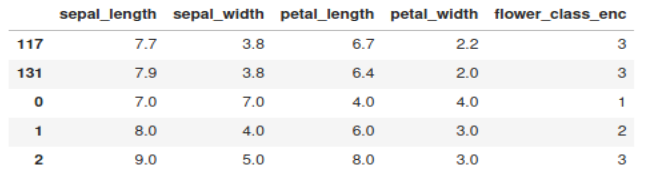
is_anomaly = scored['Loss_mae'] > scores_threshold
df_anomaly = X_train[is_anomaly]

print(df_anomaly) 

The three anomalies that we introduced in the dataset are appearing at the bottom.


Elephas Documentation: Github

Types of Artificial Neural Networks and their Applications

Supervised:

1. Simple Artificial Neural Networks: Used for Regression and Classification

2. Convolutional Neural Networks: Used for Computer Vision

3. Recurrent Neural Networks:     Used in Time Series Analysis, Natural Language Processing

Unsupervised:

1. Self-Organizing Maps:    Used for Feature Detection

2. Deep Boltzmann Machines: Used for Recommendation Systems

3. Auto-encoders:           Used for Recommendation Systems, Outlier Detection