Q1: Tell about yourself.
Q2: What all Python packages you have worked on?
Q3: What are embeddings?
Embeddings are a type of representation for text, images, or other data types that map high-dimensional inputs into lower-dimensional vector spaces. In the context of natural language processing (NLP) and machine learning, embeddings are particularly useful because they enable the representation of words, phrases, or even entire documents as dense vectors of real numbers. These vectors capture semantic meaning in such a way that similar concepts are located near each other in the embedding space.
Key Concepts of Embeddings
Dimensionality Reduction:
Embeddings reduce the dimensionality of data while preserving meaningful relationships. For example, words in a high-dimensional vocabulary are mapped to lower-dimensional vectors.
Semantic Representation:
Embeddings capture semantic similarities. Words with similar meanings are represented by vectors that are close to each other in the embedding space. For instance, the words "king" and "queen" might be close in the vector space.
Contextual Information:
Advanced embeddings like those produced by models such as BERT or GPT capture contextual information, meaning the representation of a word can change based on the surrounding words.
Types of Embeddings
Word Embeddings:
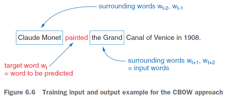
Word2Vec: Trains shallow neural networks to predict the context given the word (Skip-gram) or predict a word given the context (CBOW - Continuous Bag of Words).
Trick to remember: C for 'given the Context' and C for CBOW.
GloVe (Global Vectors for Word Representation): Combines the benefits of local context window methods and global matrix factorization methods.
FastText: An extension of Word2Vec that considers subword information, making it robust to out-of-vocabulary words.
Contextual Embeddings:
BERT (Bidirectional Encoder Representations from Transformers): Generates embeddings that consider the context of a word within a sentence. The same word can have different embeddings based on its usage.
GPT (Generative Pre-trained Transformer): Produces embeddings that are used for generating text based on a given context.
Sentence and Document Embeddings:
Doc2Vec: Extends Word2Vec to create vectors for entire documents.
Universal Sentence Encoder: Produces embeddings for sentences and paragraphs, designed to capture the meaning of longer text segments.
Image Embeddings:
Used in computer vision to represent images as vectors. These embeddings are typically generated using convolutional neural networks (CNNs).
Applications of Embeddings
Text Similarity and Search:
Embeddings are used to find similar documents or sentences by comparing their vector representations. For example, in search engines, embeddings can improve the relevance of search results.
Machine Translation:
Embeddings facilitate the translation of text from one language to another by capturing the semantic meaning of words and phrases.
Recommendation Systems:
User and item embeddings can be used to recommend products, movies, or music based on similarities in the embedding space.
Sentiment Analysis:
Embeddings can help in understanding the sentiment of a piece of text by capturing the nuanced meaning of words and phrases.
~~~
Q4: What is the difference between one-hot encoding and embeddings?
One-hot encoding and embeddings are both techniques used to represent categorical data, particularly in natural language processing (NLP) and machine learning. However, they differ significantly in their methodology, storage efficiency, and ability to capture semantic meaning.
One-Hot Encoding
Definition:
One-hot encoding is a representation of categorical variables as binary vectors. Each category or word is represented by a vector where only one element is "hot" (i.e., set to 1) and all other elements are "cold" (i.e., set to 0).
Characteristics:
Dimensionality:
The length of each one-hot vector equals the number of unique categories in the dataset. For a vocabulary of size V, each one-hot vector is of length V.
Sparsity:
One-hot vectors are sparse, containing mostly zeros except for a single 1.
No Semantic Information:
One-hot encoding does not capture any semantic relationships between categories. Each category is equidistant from every other category.
Memory Inefficiency:
For large vocabularies, one-hot encoding can be very memory-intensive due to the high dimensionality and sparsity.
Example:
For a vocabulary of {apple, banana, orange}:
apple: [1, 0, 0]
banana: [0, 1, 0]
orange: [0, 0, 1]
Definition:
Embeddings are dense vector representations of categorical data. Each category or word is mapped to a vector of fixed size, typically much smaller than the size of the vocabulary. Embeddings are learned from data and can capture semantic relationships.
Characteristics
Dimensionality:
The length of each embedding vector is much smaller than the number of unique categories, typically ranging from 50 to 300 dimensions.
Density:
Embedding vectors are dense, with most elements being non-zero.
Semantic Information:
Embeddings capture semantic meanings and relationships. Words with similar meanings have similar vectors (i.e., are close in the embedding space).
Memory Efficiency:
Embeddings are more memory-efficient compared to one-hot encoding due to their lower dimensionality.
Example:
For a vocabulary of {apple, banana, orange}, with embeddings of size 3:
apple: [0.1, 0.3, 0.5]
banana: [0.2, 0.4, 0.6]
orange: [0.0, 0.2, 0.4]
Aspect One-Hot Encoding Embeddings Dimensionality Size of vocabulary (V) Fixed size (e.g., 50-300) Vector Type Sparse Dense Semantic Information No Yes Memory Efficiency Low (due to high dimensionality) High (due to lower dimensionality) Training Requirement None (deterministic) Requires training (or pre-trained) Relationship Capture No relationships between categories Captures relationships between words
Use Cases
One-Hot Encoding:
Suitable for categorical variables with a small number of unique categories.
Often used in traditional machine learning algorithms that cannot directly handle categorical variables (e.g., decision trees, linear models).
Embeddings:
Suitable for large vocabularies, especially in NLP tasks.
Used in deep learning models such as neural networks for tasks like text classification, machine translation, and sentiment analysis.
Commonly used pre-trained embeddings include Word2Vec, GloVe, and embeddings from transformer models like BERT and GPT.
~~~
Q5: What is Count Vectorizer?
The Count Vectorizer is a technique used to convert a collection of text documents into a matrix of token counts. It is a simple and commonly used method for feature extraction in natural language processing (NLP) and text analysis. The idea is to represent each document as a vector of word counts, which can then be used as input for various machine learning algorithms.
How Count Vectorizer Works
Tokenization:
The text documents are tokenized, meaning they are split into individual words or tokens.
Building the Vocabulary:
A vocabulary (or dictionary) is built from the unique tokens across the entire corpus of documents.
Counting Tokens:
For each document, the number of occurrences of each token in the vocabulary is counted.
Vector Representation:
Each document is represented as a vector of token counts, where each element of the vector corresponds to the count of a specific token from the vocabulary.
Example
Suppose we have the following documents:
"I love programming"
"Programming is fun"
"I love machine learning"
The Count Vectorizer would perform the following steps:
Tokenization:
Document 1: ["I", "love", "programming"]
Document 2: ["Programming", "is", "fun"]
Document 3: ["I", "love", "machine", "learning"]
Building the Vocabulary:
Vocabulary: {"I", "love", "programming", "is", "fun", "machine", "learning"}
Counting Tokens:
Document 1: [1, 1, 1, 0, 0, 0, 0]
Document 2: [0, 0, 1, 1, 1, 0, 0]
Document 3: [1, 1, 0, 0, 0, 1, 1]
Advantages of Count Vectorizer
Simplicity:
Easy to understand and implement.
Efficiency:
Suitable for many text classification tasks.
Foundation for Other Techniques:
Forms the basis for more advanced techniques like TF-IDF (Term Frequency-Inverse Document Frequency).
Limitations of Count Vectorizer
Sparsity:
The resulting vectors can be very sparse, especially for large vocabularies.
Ignoring Context:
It does not consider the context or order of words, only their frequency.
High Dimensionality:
The size of the vectors increases with the size of the vocabulary, which can lead to high-dimensional data that is computationally expensive to process.
No Semantic Understanding:
Similar words or synonyms are treated as entirely separate features.
Despite these limitations, Count Vectorizer is a valuable tool for initial text processing and feature extraction in NLP pipelines.
~~~
Q6: Brief about Word2Vec?
Word2Vec is a popular technique for natural language processing (NLP) that involves training a shallow neural network model to learn dense vector representations of words. These vector representations, known as word embeddings, capture the semantic relationships between words in a continuous vector space. Developed by a team of researchers led by Tomas Mikolov at Google in 2013, Word2Vec has been influential in advancing the field of NLP.
Key Concepts of Word2Vec
Distributed Representations:
Unlike traditional one-hot encoding, which represents words as sparse vectors, Word2Vec represents words as dense vectors of real numbers. This allows the model to capture more information about the relationships between words.
Semantic Similarity:
Words with similar meanings are located close to each other in the vector space. For example, the words "king" and "queen" might have vectors that are close together, reflecting their semantic similarity.
Contextual Information:
Word2Vec captures the context of words in a corpus, which helps in understanding their meanings based on surrounding words.
Training Word2Vec
Word2Vec can be trained using two main approaches:
Continuous Bag of Words (CBOW):
In the CBOW model, the objective is to predict a target word given its context (the surrounding words). This model averages the context word vectors to predict the target word.
Skip-gram:
In the Skip-gram model, the objective is to predict the context words given a target word. This model is particularly effective for smaller datasets and captures more fine-grained information about word relationships.
Applications of Word2Vec
Similarity and Analogy Tasks:
Word2Vec can be used to find similar words and perform analogy tasks. For example, finding the word that is to "queen" as "king" is to "man".
Text Classification:
Embeddings from Word2Vec can be used as features in text classification tasks, such as sentiment analysis or spam detection.
Advantages of Word2Vec
Semantic Understanding:
Captures semantic relationships between words, making it useful for various NLP tasks.
Efficient Training:
Word2Vec is computationally efficient and can be trained on large datasets relatively quickly.
Flexibility:
Can be fine-tuned for specific tasks and integrated into larger machine learning pipelines.
Limitations of Word2Vec
Context Independence:
Word2Vec generates a single vector representation for each word, regardless of its context in a sentence. This can be a limitation for words with multiple meanings (polysemy).
Static Embeddings:
The embeddings are static once trained and do not change with new data unless retrained.
Requires Large Datasets:
To capture meaningful relationships, Word2Vec requires a large corpus for training.
~~~
Q7: Brief about the Architecture of Word2Vec.
Skip-Gram model:


 Continuous Bag of Words:

 ~~~
Q8: Brief about Anomaly detection and following three types of models that you tried:
- Auto encoder
- K-medians
- Isolation Forest
~~~
Q9: Provide the End-to-end project description for the Anomaly Detection project.
~~~
Q10: Is it correct to say if maximise negative of log-likelihood of an observation to detect anomalies?
Maximizing the negative log-likelihood of an observation is not typically used for anomaly detection. Instead, minimizing the negative log-likelihood is more common in training machine learning models. To detect anomalies, one would often look for observations that have low likelihoods (or high negative log-likelihoods) under a given model, rather than maximizing the negative log-likelihood.
Understanding Negative Log-Likelihood (NLL)
Log-Likelihood:
In a probabilistic model, the likelihood of an observation is the probability of the observation given the parameters of the model.
The log-likelihood is simply the natural logarithm of the likelihood. Taking the logarithm helps in dealing with very small probability values and can simplify the differentiation process during optimization.
Negative Log-Likelihood:
The negative log-likelihood (NLL) is the negative of the log-likelihood. Minimizing the NLL is equivalent to maximizing the likelihood.
In many machine learning models, such as neural networks, we minimize the NLL during training to find the best model parameters.
Anomaly Detection
In anomaly detection, the goal is to identify observations that deviate significantly from the normal behavior captured by the model. Here’s how the concept of log-likelihood can be applied:
Train a Probabilistic Model:
Train a model on normal (non-anomalous) data to capture the distribution of normal behavior.
Compute Log-Likelihoods:
For each new observation, compute the log-likelihood under the trained model.
Identify Anomalies:
Observations with low likelihoods (equivalently, high negative log-likelihoods) are considered anomalies. These are points that the model considers unlikely under the learned distribution of normal data.
Example
Consider a Gaussian Mixture Model (GMM) for anomaly detection:
Train GMM on Normal Data:
python
Copy code
from sklearn.mixture import GaussianMixture
# Assume X_train contains normal data
gmm = GaussianMixture(n_components=2).fit(X_train)
Compute Log-Likelihoods:
python
Copy code
# Assume X_test contains new observations
log_likelihoods = gmm.score_samples(X_test)
Detect Anomalies:
python
Copy code
# Set a threshold for anomaly detection
threshold = -10
anomalies = X_test[log_likelihoods < threshold]
In this example, gmm.score_samples(X_test) returns the log-likelihood of each observation in X_test. Observations with log-likelihoods below the threshold are considered anomalies.
~~~
Q8: Brief about Anomaly detection and following three types of models that you tried:
- Auto encoder
- K-medians
- Isolation Forest
~~~
Q9: Provide the End-to-end project description for the Anomaly Detection project.
~~~
Q10: Is it correct to say if maximise negative of log-likelihood of an observation to detect anomalies?
Maximizing the negative log-likelihood of an observation is not typically used for anomaly detection. Instead, minimizing the negative log-likelihood is more common in training machine learning models. To detect anomalies, one would often look for observations that have low likelihoods (or high negative log-likelihoods) under a given model, rather than maximizing the negative log-likelihood.
Understanding Negative Log-Likelihood (NLL)
Log-Likelihood:
In a probabilistic model, the likelihood of an observation is the probability of the observation given the parameters of the model.
The log-likelihood is simply the natural logarithm of the likelihood. Taking the logarithm helps in dealing with very small probability values and can simplify the differentiation process during optimization.
Negative Log-Likelihood:
The negative log-likelihood (NLL) is the negative of the log-likelihood. Minimizing the NLL is equivalent to maximizing the likelihood.
In many machine learning models, such as neural networks, we minimize the NLL during training to find the best model parameters.
Anomaly Detection
In anomaly detection, the goal is to identify observations that deviate significantly from the normal behavior captured by the model. Here’s how the concept of log-likelihood can be applied:
Train a Probabilistic Model:
Train a model on normal (non-anomalous) data to capture the distribution of normal behavior.
Compute Log-Likelihoods:
For each new observation, compute the log-likelihood under the trained model.
Identify Anomalies:
Observations with low likelihoods (equivalently, high negative log-likelihoods) are considered anomalies. These are points that the model considers unlikely under the learned distribution of normal data.
Example
Consider a Gaussian Mixture Model (GMM) for anomaly detection:
Train GMM on Normal Data:
python
Copy code
from sklearn.mixture import GaussianMixture
# Assume X_train contains normal data
gmm = GaussianMixture(n_components=2).fit(X_train)
Compute Log-Likelihoods:
python
Copy code
# Assume X_test contains new observations
log_likelihoods = gmm.score_samples(X_test)
Detect Anomalies:
python
Copy code
# Set a threshold for anomaly detection
threshold = -10
anomalies = X_test[log_likelihoods < threshold]
In this example, gmm.score_samples(X_test) returns the log-likelihood of each observation in X_test. Observations with log-likelihoods below the threshold are considered anomalies.
Summary
Training Phase: Minimize negative log-likelihood to learn model parameters.
Detection Phase: Identify anomalies by looking for observations with low likelihoods (high negative log-likelihoods).
Therefore, it is not correct to say that maximizing the negative log-likelihood of an observation is used to detect anomalies. Instead, we use the concept of likelihood (or log-likelihood) to find observations that are unlikely under the model and thus potential anomalies.
~~~
Q11: What is ginie index?
The Gini index, also known as the Gini impurity, is a metric used to evaluate the quality of a split in decision tree algorithms, such as CART (Classification and Regression Trees). It measures the degree of impurity or diversity in a dataset. The lower the Gini index, the less impure the node is, meaning that it is more homogenous.
Definition
The Gini index for a node is defined as:
where:
- is the number of classes.
- is the proportion of instances of class in the node.
Interpretation
- Gini Index of 0:
- Indicates a pure node, where all instances belong to a single class.
- Gini Index of 0.5:
- Indicates a completely impure node, where the instances are uniformly distributed across all classes (in the case of two classes).
Example Calculation
Suppose we have a node with the following class distribution:
- Class A: 3 instances
- Class B: 2 instances
The total number of instances is 5. The proportions are:
The Gini index for this node is:
Usage in Decision Trees
In decision tree algorithms, the Gini index is used to select the best feature to split the data at each node. The algorithm chooses the feature that minimizes the weighted sum of the Gini indices of the child nodes, effectively selecting the split that produces the most homogenous child nodes.
Pseudocode for Gini Index in Decision Tree Split
pythondef gini_index(groups, classes):
# Count all samples at split point
n_instances = float(sum([len(group) for group in groups]))
# Sum the Gini index for each group
gini = 0.0
for group in groups:
size = float(len(group))
# Avoid division by zero
if size == 0:
continue
score = 0.0
# Score the group based on the score for each class
for class_val in classes:
p = [row[-1] for row in group].count(class_val) / size
score += p * p
# Weight the group score by its relative size
gini += (1.0 - score) * (size / n_instances)
return gini
In this pseudocode:
groups is a list of groups formed by splitting the dataset on a particular feature.classes is a list of unique class values in the dataset.- The function calculates the Gini index for each group and returns the weighted sum of the Gini indices.
Conclusion
The Gini index is a fundamental concept in decision tree learning, used to evaluate the quality of splits and guide the tree-building process. By selecting splits that minimize the Gini index, decision trees aim to create nodes that are as pure as possible, leading to more accurate and interpretable models.
~~~
Q12: How do you do attribute selection for building a decision tree?
Attribute selection for building a decision tree involves choosing the most informative features to split the data at each node in the tree. The goal is to select attributes that maximize the purity of the child nodes, thus improving the decision tree's ability to correctly classify the data. The most commonly used criteria for attribute selection in decision trees are Gini Index, Information Gain, and Gain Ratio.
Steps in Attribute Selection
Calculate the Splitting Criteria for Each Attribute:
Gini Index: Measures the impurity of a dataset. Lower values indicate purer nodes.
Information Gain: Measures the reduction in entropy (disorder) after a dataset is split on an attribute.
Gain Ratio: Adjusts the information gain by taking into account the intrinsic information of a split, addressing the bias towards attributes with many values.
Choose the Attribute with the Best Split:
Select the attribute that either minimizes the Gini Index or maximizes the Information Gain or Gain Ratio.
Repeat the Process for Child Nodes:
Recursively apply the attribute selection process to the child nodes until stopping criteria are met (e.g., maximum tree depth, minimum number of samples per leaf, or no further information gain).
~~~
Q13: Which ones are faster Boosting algorithms or Bagging Algorithms?
In general, Bagging algorithms tend to be faster than Boosting algorithms. Here’s a detailed comparison of both techniques in terms of speed and computational complexity:
Bagging Algorithms
Characteristics:
Parallel Training: Bagging (Bootstrap Aggregating) algorithms train multiple base learners (e.g., decision trees) independently in parallel. Each learner is trained on a different bootstrap sample of the training data.
Less Sequential Dependency: Since each base learner is trained independently, the overall training process can be parallelized, making it faster and more efficient.
Examples: Random Forest is a common example of a bagging algorithm.
Speed:
Training Speed: Bagging is generally faster because each model can be trained independently and in parallel.
Prediction Speed: Bagging can also be faster during prediction because the models are independent, and predictions from each model can be averaged in parallel.
Boosting Algorithms
Characteristics:
Sequential Training: Boosting algorithms train base learners sequentially. Each new learner is trained to correct the errors made by the previous learners.
High Sequential Dependency: The training of each base learner depends on the performance of the previous learners, leading to a more sequential and thus slower process.
Examples: AdaBoost, Gradient Boosting Machines (GBM), XGBoost, and LightGBM are common examples of boosting algorithms.
Speed:
Training Speed: Boosting is generally slower due to the sequential nature of training. Each new model needs to be trained based on the performance of the previous model, which prevents parallel training.
Prediction Speed: Boosting can also be slower during prediction because the predictions are made sequentially by each model in the boosting chain.
Detailed Comparison
1. Training Speed
Bagging: Faster training due to parallelism. All base models are trained independently, and the process can take advantage of multiple CPU cores or distributed computing.
Boosting: Slower training because models are built sequentially. Each model corrects the errors of the previous ones, preventing parallel training.
2. Prediction Speed
Bagging: Predictions can be made relatively quickly because each model's prediction can be computed in parallel and then averaged or voted upon.
Boosting: Predictions can be slower because they involve sequentially aggregating the results of all models in the boosting chain.
3. Scalability
Bagging: More scalable due to parallelizable nature, especially beneficial for large datasets and distributed computing environments.
Boosting: Less scalable due to the sequential dependency of the models.
Summary
Bagging algorithms (e.g., Random Forest) are generally faster in both training and prediction phases due to their parallelizable nature.
Boosting algorithms (e.g., XGBoost, LightGBM) are typically slower due to the sequential training process and the dependency of each model on the performance of the previous ones.
However, it’s important to note that boosting algorithms often achieve higher accuracy and better performance on certain tasks due to their sequential learning process and the focus on correcting errors from previous models. The choice between bagging and boosting should depend on the specific requirements of your problem, including the trade-offs between speed and accuracy.
~~~
Q14: What is confusion matrix?
A confusion matrix is a performance measurement tool for machine learning classification problems. It is a table that is used to describe the performance of a classification model (or "classifier") on a set of test data for which the true values are known. The confusion matrix itself is relatively simple to understand, but the terminology can be a bit confusing.
Components of a Confusion Matrix
A confusion matrix for a binary classifier is a 2x2 matrix with the following structure:
Predicted Positive Predicted Negative
Actual Positive True Positive (TP) False Negative (FN)
Actual Negative False Positive (FP) True Negative (TN)
For a multi-class classification problem, the matrix would be larger, with dimensions corresponding to the number of classes.
Definitions
True Positive (TP): The number of correct positive predictions.
True Negative (TN): The number of correct negative predictions.
False Positive (FP): The number of incorrect positive predictions (also known as Type I error).
False Negative (FN): The number of incorrect negative predictions (also known as Type II error).
~~~
Q15: When do you use Precision and when do you use Recall? Provide an example.
Answer:
Precision and recall are two important metrics used to evaluate the performance of classification models, especially in contexts where class distribution is imbalanced or where the costs of false positives and false negatives differ significantly.
Precision
Definition: Precision measures the proportion of true positive predictions out of all positive predictions made by the model.
When to Use:
- High Cost of False Positives: When the cost of incorrectly labeling a negative instance as positive is high, precision is crucial. For example, in medical diagnostics, false positives (e.g., diagnosing a healthy person with a disease) can lead to unnecessary stress and additional testing.
- Precision-Oriented Tasks: When you need to ensure that the positive predictions you make are highly reliable.
Example: Suppose you are developing a spam email filter. Precision is important if you want to avoid marking legitimate emails as spam. A high precision means that when your model classifies an email as spam, it is likely to be spam.
Recall
Definition: Recall measures the proportion of true positive predictions out of all actual positives in the dataset.
When to Use:
- High Cost of False Negatives: When missing positive instances is costly or dangerous, recall is crucial. For example, in cancer screening, a false negative (failing to detect a disease when it is present) can have severe consequences.
- Recall-Oriented Tasks: When you want to capture as many positive instances as possible, even if it means including some false positives.
Example: In a disease outbreak detection system, recall is crucial to ensure that as many actual cases as possible are detected, even if it means some healthy individuals might be incorrectly flagged as potentially infected.
Example Scenario
Scenario: Consider a model designed to identify fraudulent transactions in a banking system.
Precision: If the model has high precision, it means that when it flags a transaction as fraudulent, it is likely to be fraudulent. This is important to reduce the number of legitimate transactions mistakenly flagged as fraud, which can cause inconvenience for customers.
Recall: If the model has high recall, it means it detects a high proportion of all fraudulent transactions. This is important to ensure that as many fraudulent activities as possible are caught, even if it means flagging some legitimate transactions as fraudulent.
Trade-Off Between Precision and Recall
In many cases, there is a trade-off between precision and recall. Improving one often reduces the other. For example, setting a higher threshold for classifying a transaction as fraudulent will increase precision (fewer legitimate transactions are incorrectly classified as fraud) but may decrease recall (some fraudulent transactions might be missed).
Balancing Act:
- F1 Score: To balance precision and recall, you can use the F1 score, which is the harmonic mean of precision and recall. It provides a single metric that considers both false positives and false negatives.
Summary
- Use Precision: When false positives are costly and you want to ensure that positive predictions are reliable.
- Use Recall: When false negatives are costly and you want to capture as many positive instances as possible.
Choosing the appropriate metric depends on the specific context and the costs associated with false positives and false negatives in your application.
~~~
Q16: Calculate precision and recall for this given confusion matrix.
~~~
Q17: How many jumps it would take to climb a 100 storey building if you double your strength with every jump? And you start with 1 storey a jump.
To determine how many jumps it would take to climb a 100-storey building if you double your strength with each jump, starting with the ability to jump 1 storey on the first jump, we can use the concept of geometric progression.
Understanding the Problem
- Initial Jump Strength: 1 storey (on the first jump)
- Doubling Factor: After each jump, the jumping strength doubles.
Calculation
- Jump 1: You jump 1 storey.
- Jump 2: You jump storeys.
- Jump 3: You jump storeys.
- Jump 4: You jump storeys.
And so on. The number of storeys you can jump after jumps is given by .
To find the number of jumps required to reach or exceed 100 storeys, we need to find the smallest such that:
The sum of the first terms of a geometric series is:
So we need:
Solving for :
Find such that:
Calculate powers of 2 to find the smallest :
- (not enough)
- (sufficient)
So, is the smallest integer satisfying .
Conclusion
It would take 7 jumps to climb a 100-storey building if you double your jumping strength with each jump, starting from 1 storey on the first jump.
~~~
Q18: Which all cloud platforms you have used?
Q19: What is Delta Table in Databricks?
Delta Table is a key feature of Delta Lake, which is an open-source storage layer developed by Databricks to bring ACID (Atomicity, Consistency, Isolation, Durability) transactions and scalable metadata handling to big data workloads. Delta Lake is built on top of existing data lakes (like Apache Spark and Apache Hive) and provides a unified approach to handling streaming and batch data.
Key Features of Delta Tables
ACID Transactions: Delta Tables support ACID transactions, which ensure that all operations are completed successfully or none are applied, maintaining data integrity. This is crucial for handling concurrent writes and reads.
Schema Evolution and Enforcement: Delta Tables allow schema evolution, which means you can modify the schema of the table (add or remove columns) without rewriting the entire dataset. Schema enforcement ensures that the data adheres to the defined schema.
Time Travel: Delta Tables support time travel, which lets you query historical versions of the data. This feature is useful for auditing, data recovery, and reproducing experiments.
Upserts and Deletes: Delta Tables support upserts (merge operations) and deletes, which are not natively supported by traditional data lakes like HDFS. This enables efficient data updates and deletions.
Scalable Metadata Handling: Delta Lake handles metadata at scale efficiently, which is beneficial for large-scale data processing. It avoids the performance bottlenecks associated with traditional data lakes.
Data Optimization: Delta Tables provide built-in data optimization features such as data skipping and file compaction, which improve query performance by reducing the amount of data read.
Delta Table Architecture
Delta Tables are built on top of existing file formats (e.g., Parquet) and add a transaction log to manage changes. The architecture includes:
Data Files: Actual data is stored in Parquet files or other file formats.
Transaction Log: A Delta Log (stored as a series of JSON files) tracks all changes to the table. It contains metadata about the table, including schema changes, additions, deletions, and data modifications.
Checkpoint Files: Periodic snapshots of the transaction log are saved to improve read performance and recovery times.
Basic Operations with Delta Tables
Here’s how you typically interact with Delta Tables using Databricks:
Create a Delta Table:
CREATE TABLE delta_table
USING DELTA
AS SELECT * FROM source_table;
Write Data to a Delta Table:
df.write.format("delta").mode("append").save("/path/to/delta_table")
Read Data from a Delta Table:
df = spark.read.format("delta").load("/path/to/delta_table")
Update Data in a Delta Table:
from delta.tables import DeltaTable
delta_table = DeltaTable.forPath(spark, "/path/to/delta_table")
delta_table.alias("t").merge(
source_df.alias("s"),
"t.id = s.id"
).whenMatchedUpdate(set={"value": "s.value"}) \
.whenNotMatchedInsert(values={"id": "s.id", "value": "s.value"}) \
.execute()
Time Travel:
df = spark.read.format("delta").option("timestampAsOf", "2023-01-01").load("/path/to/delta_table")
Optimize and Vacuum:
delta_table.optimize()
delta_table.vacuum(retentionHours=168)
Conclusion
Delta Tables provide a robust and flexible framework for managing data in a data lake, combining the advantages of traditional data lakes with features that support ACID transactions, schema evolution, and efficient metadata management. This makes them a powerful tool for handling large-scale data processing and analytics workloads in Databricks.